 Graziano & Raulin
Research Methods (9th edition)
Analyzing Categorical Data
Categorical data are analyzed with a procedure called chi square. In this unit, we will be using chi square in two different ways. In the first procedure, we will be comparing the pattern of frequencies against a hypothesized pattern. This procedure is called the chi square goodness-of-fit test. It is conceptually equivalent to the single-group t-test, in which we compared our single sample against a hypothesized population mean.
In the second procedure, we will be comparing two or more groups to see if the pattern of frequencies varies from group to group. This procedure is called the chi square test for independence. It is conceptually equivalent to the two-group t-test or one-way ANOVA, in which we compare two or more groups on the mean scores of the groups.
Chi Square Goodness-of-Fit Test
The chi square goodness-of-fit test compares that pattern of frequencies against a hypothesized pattern. For example, we might want to evaluate the honesty of a coin by flipping it 50 times and comparing the pattern of heads and tails against what we would expect if the coin were honest (50% heads and 50% tails).
Suppose that we find that in 50 flips of a coin, we get 31 heads and 19 tails. That is 12 more heads than tails in our 50 flips of the coin. Is that deviation from the 25/25 split we would expect of an honest coin so large that we would question the honesty of the coin? What do you think?
Clearly, if we flip an honest coin 50 times, we expect 50% heads on average, but any block of 50 might deviate from that 50% due to chance, which is the conceptual equivalent of the sampling error that we discussed when we talked about parametric statistics. We need a way to decide how far from our 25/25 split is likely in a coin that is honest, and the chi square goodness-of-fit test gives us a way to evaluate such questions.
We start by organizing our data into a matrix, as shown below. We list the categories across the top (heads and tails), and along the side we list both the observed frequencies and the expected frequencies. The expected frequencies are based on a specific hypothesis. In our example, we are assuming the the coin is honest, so that we expect a 50%/50% split of heads and tails. However, we might have situations in which our hypothesis might be more complex. For example, if each trial involved flipping two coins and counting the number of heads, we would expect 25% of the time to get zero heads, 50% of the time to get 1 head, and 25% of the time to get two heads if the coins are honest. [If you are having trouble figuring out why that should be the case, you may want to review the section on probability.]
|
Heads |
Tails |
|
| Observed Frequency | 31 | 19 |
| Expected Frequency | 25 | 25 |
Note that the sum of the observed frequency must equal the sum of the expected frequency. In fact, we compute the expected frequencies by multiplying the expected proportions by the observed frequencies. In our case, we expect a 50%/50% split between heads and tails (.50/.50 expressed as a proportion). So we multiply .50 times 50 (our total observed frequency) to get 25 heads and 25 tails.
The equation for computing the chi square goodness of fit is shown below. The values of Oi and Ei are the observed and expected frequencies for each possible category (k is the number of categories). We plug in those numbers as shown in the equation and then sum across the categories, as shown below.
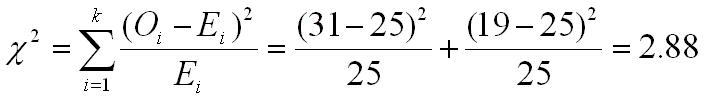
To evaluate the computed value of chi square, we need to compare it to a critical value in exactly the same way that we have done for other statistical tests. We look up the critical value in the chi square table using our selected value of alpha and the degrees of freedom. The degrees of freedom in the goodness-of-fit test are the number of categories minus 1 (k-1), which in this case is equal to 1. If you consult the table for an alpha of .05 and df of 1, you will find the the critical value of chi square is 3.841. The computed value of chi square does not exceed this value. Therefore, we fail to reject the null hypothesis and conclude that the coin could be honest and still give the 31/19 split that we found.
Are you surprised? Many people see a 31/19 split of 50 flips of a coin as so unusual that it must mean that the coin is not honest, but statistical procedures tell us such a result it not all that rare.
You can see another example of computing a chi square goodness-of-fit test by hand by clicking the top button below. You can also see how you would compute the same test using SPSS for Windows by clicking the second button.
|
Compute a Chi Square Goodness of Fit Test by hand |
|
Compute a Chi Square Goodness of Fit Test using SPSS |
|
USE THE BROWSER'S |
Common Mistakes with Chi Square
There are three common mistakes that students make in computing chi square. We will illustrate the first two using the example above, but will need to use a different example to illustrate the third.
The data for chi square computations should always be frequencies, never percentages. Let's make the mistake of using percentages instead of frequencies with the coin flipping example above and see what happens. The table will change as shown below, and the changes in the table will result in the changes in the chi square shown below.
|
Heads |
Tails |
|
| Observed Percentages | 62 | 38 |
| Expected Percentages | 50 | 50 |
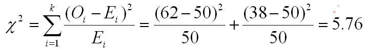
The chi square this time is 5.76. The degrees of freedom is unchanged, so the critical value of chi square for an alpha of .05 is still 3.841. So our conclusion would be that our data suggests that our coin is biased, which is just the opposite conclusion that we came to based on our original analysis.
What is happening here? By using percentages instead of the original frequencies, we are acting as if our sample size was 100 trials instead of the 50 trials that we actually conducted. Remember the concept that we established when we first talked about estimating population means. The larger the sample size, the closer we can expect our sample mean to be, on average, to the population mean. We have the same phenomenon occurring in this example.
If we flipped a coin 5 times and got 3 heads (close to the 62% we found in the 50 trial test), we would recognize that this is pretty weak evidence for a biased coin. In fact, the coin could not get any closer to the 50% split we are hypothesizing. If we flipped the coin 10 times and got 6 heads, we would realize that if just one of the heads had been a tails instead, it would have been exactly a 50%/50% split. So again we would realize that this is pretty weak evidence for a biased coin. The 31/19 split that we got in the example of flipping the coin 50 times starts to make us suspicious, even though the percentages are roughly the same. The chi square tells us that one could get such figures by chance alone, so we would not conclude that the coin was dishonest. However, getting those percentages with 100 trials is extremely unlikely if the coin is honest.
The more trials we conduct (i.e., the larger the sample size) the closer our data should be to the population value. If the coin is honest, we can expect that the more times we flip it, the closer our proportion should be to the hypothetical 50%/50% breakdown we expect from an honest coin. So remember, you must use frequencies in your chi square computations.
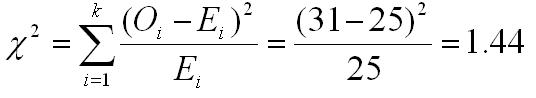
The second error that is commonly made by students is to not include all of the possible categories in the analysis. Every single trial must fit into a category and all of the categories must be included in the analysis. Statisticians would say that the categories must be exhaustive, which means that they represent every possible outcome, even if it never occurs. Let's use a use a variation on the above example to illustrate this problem. When we flip a coin, we have two possibilities (heads and tails), and both must be represented in our data matrix to do the chi square correctly. If we flip the coin 50 times and get 31 heads, it means that we also got 19 tails. However, if we set up the matrix and forget to include the tails category, it would like the matrix below.
| Heads | |
| Observed Frequency | 31 |
| Expected Frequency | 19 |
Now if we compute the value of chi square, we get 1.44, which is clearly different from what we got when we include both the heads and the tails categories.
Now leaving off the tails category may seem like the kind of error that no one would make, but this is actually a fairly common error. For example, if you obtain data from participants on their political affiliation, every person you ask MUST fit into one of your categories. So if your categories are Democrat, Republican, and Independent, you have a problem if a participant says he or she is in the Green Party or the Socialist Party or has no political affiliation. To handle this problem, the norm is to have a category for everyone who does not fit into the primary categories. In this case, it might be Other, which could include any other party affiliation or no party affiliation.
Finally, every individual who is part of a chi square analysis can contribute one and ONLY one data point. Another way of saying this is that the categories must be mutually exclusive. That means that one must be very careful about setting up the categories for a chi square analysis.
For example, it might seem perfectly reasonable to have the categories of single, married, divorced, and widowed for marital status, but how do you categorize someone who is a widower that remarried or someone who remarried following a divorce or someone who is not married, but divorced one spouse and lost a second spouse to cancer. Clearly, these are not mutually exclusive categories, and therefore this breakdown is inappropriate for a chi square analysis. However, with a little thought we could make them mutually exclusive. For example, we could have the categories single and never married, married, currently single but previously married. This is a set of marital status categories that is both exhaustive and mutually exclusive.
Chi Square Test for Independence
The chi square test for independence is a way of comparing two or more groups on the distribution of individuals in those groups into a set of exhaustive categories.
For example, you might want to compare men and women on the primary car that they drive. The categories are (1) small to midsize auto, (2) SUV, (3) luxury vehicle, (4) truck, and (5) other (includes none). These categories were designed to be both exhaustive and mutually exclusive. Suppose we get the following data when we interview a group of men and women.
| Small to Midsize | SUV | Luxury | Truck | Other | Totals | |
| Women | 26 | 36 | 6 | 13 | 16 | 97 |
| Men | 21 | 19 | 12 | 21 | 5 | 78 |
| Totals | 47 | 55 | 18 | 34 | 21 | 175 |
We use the same formula for computing a chi square test for independence as you use for computing a chi square goodness-of-fit test. The only difference is how the excepted cell frequencies are computed.
In the goodness-of-fit test, the expected cell frequencies are a function of our hypothesis. For example, if we hypothesize that the coin is honest, we expect half of your flips to be heads and half to be tails. In contrast, with the test for independence, we use the pattern of scores to produce the expected cell frequencies. To do this, we create row and column totals as well as a grand total. Then we compute the expected cell frequency for each cell by multiplying the row total for that cell by the column total for that cell and dividing by the grand total.
For example, in the table above, we would compute the expected cell frequency for the cell that represents the number of women driving a small to midsize car by multiplying 47 (the column total) by 97 (the row total) and dividing by 175 (the grand total). This process is spelled out in more detail in the instructions for computing the Test for Independence by hand (click the top button below).
What this process for computing expected cell frequencies does is it produces the pattern of scores that you would get if the distribution of categories among the groups was the same in all groups. Using our example, 26 of our 97 women drove a small to midsize car. However, if the likelihood of driving a small to midsize car were the same in both mean and women, we would expect about 27% to be driving a small to midsize car (47 divided by 175). If 27% of the 97 women drove such a car, that would be about 26 women (we will ignore the numbers after the decimal point for this illustration). In other words, for this cell, we have an expected cell frequency that is virtually identical to the observed cell frequency. But let's look at the cell representing luxury cars driven by men. The observed cell frequency is 12, but the expected cell frequency is approximately 8 (18*78/175).
You can see how to compute a chi square test for independence by clicking on either of the buttons below.
|
Compute a Chi Square Test for Independence by hand |
|
Compute a Chi Square Test for Independence using SPSS |
|
USE THE BROWSER'S |