 Graziano & Raulin
Research Methods (9th edition)
Inferential Statistics
In this section, we will pause and review the various concepts that we have developed so far, organizing them into the conceptual basis for inferential statistics. This will prepare you for the next section, in which we introduce the various statistical procedures for testing a wide range of basic research hypotheses.
Populations and Samples
Scientists want to understand how things work in the world, which means that they are interested in the characteristics of large populations. Realistically, it is impossible to study such large groups, so the approach that scientists take is to study a smaller group that represents the population. By detailing the characteristics of that group or the response of that group to an intervention, scientists can draw conclusions about what would be found if the entire population could have been studied.
The science of psychology relies heavily on statistical analysis, because there are large natural differences among people on the variables that we study, such as memory, aggression, friendliness, or rate of development. Unlike other sciences, these individual differences among people are largely out of the researcher's control. For example, in chemistry, it is possible to purify chemicals so that any two samples will be exactly alike. Consequently, mixing two pure chemicals will reliably produce exactly the same reaction, with the same outcome, each time the study is performed. Such control is impossible in psychology. In fact, in some sciences, even the idea of having variables that are uncontrolled is upsetting to the scientists. Einstein's famous quotation about God not playing dice with the universe was his reaction to quantum mechanics, which argued that we can never know where an electron is, but rather can only know the probability of where it is.
Probability and Distributions
Because there are individual differences among people in any population, a sample of people drawn from the population will not always represent the population perfectly. The normal variation among samples drawn from the same population is referred to as sampling error, although this is a misleading term.
The term sampling error implies that something was done wrong in the sample, when in fact, perfect random sampling will result in sampling error. We used a better term earlier to refer to this natural variability of sample means, which we called the sampling distribution of the means, which is also called the standard error of the means or simply the standard error. (This is where the sampling error term came from.)
You learned that this sampling distribution is predictable. The mean of the sampling distribution of means is the population mean, and the variability is a function of the variability of the population and the size of the sample. The larger the sample, the smaller the variability will be, because large samples give more accurate estimates of the population mean. What that indicates is that the means will cluster more tightly around the population mean in the sampling distribution of means when the samples are large. Finally, we even know the shape of the distribution if the sample size is large. The Central Limit Theorem tells us that samples that are reasonably large will have a distribution of the means that is normal, regardless of the shape of the population distribution.
You also learned that any distribution can be thought of as a probability distribution. We can compute the relative areas under the curve and treat them as probabilities. For example, one can compute a percentile rank based on a distribution of scores that is normal. We actually can compute any conceivable area under a curve with a known shape. For example, we could compute the probability of scoring between any two scores if we know the mean and standard deviation of a normal distribution.
In general, the distribution that we will be using in inferential statistics is the distribution of means or the distribution of some combination of means. You will see examples of each of those situations in later sections. We will be asking questions like whether our sample is likely to have come from a population with a specific population mean and standard deviation. If our sample mean is close to the population mean, we will assume that it does come from the population, but the question of how close is close will be defined by the sampling distribution of the mean and the likelihood that our sample mean came from that sampling distribution.
The Null Hypothesis
The null hypothesis is a central concept in inferential statistics. It is the hypothesis that says that there is no difference. We are being deliberately vague here, because there are many different types of null hypotheses, depending on the statistical question you want to ask. The only thing that they have in common is that they all state that there is no difference between two or more quantities.
This concept is confusing to most students for two reasons. The first is that we are not really asking if there is no difference between two values, but rather whether the difference that we find is so small that it suggests that there is no difference in the population. Remember, we are using inferential statistics to draw conclusions about populations based on samples, so if the sample means are very similar, we would tend to conclude that the population means are also similar.
The second is that the null hypothesis is stated in exactly the opposite direction of what we are hoping to find. We are not looking to find no difference, but rather are predicting that there will be a difference. For example, when we treat some people who have an illness using a drug we think might work, and we compare the effectiveness of the drug to a placebo, we are expecting, or at least predicting, that the people taking the drug will show more symptom relief than the people not taking the drug.
The tradition in statistics is to label the null hypothesis as H0 (an H with a subscript of zero). The alternative hypothesis is labeled H1. The exact null and alternative hypotheses will depend on the type of statistical test that we are conducting, and you will see examples of several different null hypothesis in later sections of this statistical concepts unit.
For the purpose of illustration, let's assume that we are testing two conditions in an experiment. For example, we might be interested in whether a certain drug enhances sexual activity in rats. Psychologists study lots of interesting things like that. We have two conditions: (1) giving the drug to the rats and (2) giving the rats a placebo drug. You will learn in the text that it is desirable to have the conditions of an experiment as similar as possible to avoid confounding. Therefore, we would not want to give some rats the drug (usually through injection) and give other rats nothing. Then the groups would differ not only on the drug, but also on whether they received an injection, and this could be a source of confounding. So our groups are the drug group and the placebo group.
We want to see if they are different, but what we are really testing is whether the populations of rats who either (1) receive the drug or (2) do not receive the drug are different, and we will make this decision on the basis of how large the difference between the means are for the two samples that we are testing. This is an important distinction, because our null hypothesis always involves population parameters. Remember from our section on notation, we use the Greek letter mu to indicate a population mean. So our null and alternative hypotheses would be written as follows:
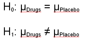
The null hypothesis is that the population means for the Drug and Placebo condition are equal (i.e., there is no effect of the drug), and the alternative hypothesis is that they are not equal. (The equal sign with a line drawn through it means "not equal.") Every statistical test that we cover in this section will have a null and alternative hypothesis similar to the ones shown in this example.
Decisions and Their Costs
We will set up a null hypothesis with every statistical hypothesis that we test. We then will compute the appropriate inferential statistic to test that hypothesis. You will see several examples of this process in later sections. The null hypothesis is always tested in the same way. If the obtained inferential statistic is unlikely to have occurred if the null hypothesis were true, we reject the null hypothesis. In other words, we conclude that the null hypothesis is false.
But how do statisticians define "unlikely to have occurred"? We use a decision criterion that is called alpha and is indicated by the Greek letter alpha. By tradition, alpha is set at a small number, usually .05, but sometimes as small as .01. If alpha is set at .05, we would reject the null hypothesis ONLY if the obtained inferential statistic has less than a 5% chance of occurring if the null hypothesis were true. That means that the null hypothesis is not rejected lightly. There has to be little chance that it is true before it is rejected, and if the alpha is set at .01, there has to be almost no chance of it being true before it is rejected.
Although the decision on the null hypothesis is made on the basis of probability, once a decision is made, you have essentially four possible outcomes, which are defined by two elements. The first element is the decision, which is either rejecting or not rejecting the null hypothesis. The second is the actual state of affairs, which is either the null hypothesis is true or it is not. These options are illustrated in the table below.
Decision |
||
Reality |
Reject
|
Fail to Reject
|
Null Hypothesis
|
Type I Error |
correct decision |
Null Hypothesis
|
correct decision |
Type II Error |
Note two things about this matrix of decisions and their effects. There are two types of errors that are possible. Type I error is rejecting the null hypothesis when it is actually true. We control Type I error, because its probability of occurring is the alpha level that we set. If we set alpha to .05, then 5% of the time we will incorrectly reject the null hypothesis.
Researchers generally prefer to set alpha low (.05 or less), because they do not want to reject the null hypothesis unless the evidence for doing so is strong. The reason for setting alpha low is a conservative bias. We are not talking about political affiliations here, but rather are talking about the principle that you do not reject established procedures unless there is strong evidence that the new procedures are superior. In most research studies, rejecting the null hypothesis involves saying that one procedure is better than another, and thus might be used as an argument for changing procedures. But changing procedures, even if you think the new procedure has proved itself superior, is costly, time consuming, and has potential risks. For example, the new procedure may be superior to the old procedure in some ways, but may have unknown risks that may not become apparent for years.
You might think that if alpha is the level of Type I error and you can set alpha at any level you like, then why not set alpha at zero and not make any Type I errors. Think about that for a minute. Setting alpha to zero is essentially saying that you will never reject the null hypothesis. But sometimes the null hypothesis is false and should be rejected. If you fail to reject it in those circumstances, you have made another error, called a Type II error. Type II error is indicated by the Greek letter beta. If nothing else changes, the level of Type II error will increase as the level of Type I error decreases. Consequently, we are balancing these two types of errors.
There is a way to decrease Type II error without changing the level of Type I error. Increasing the sample size will increase the precision of our measurement. Therefore, it will be easier to detect a small difference that might indicate that the null hypothesis is false. Statisticians use the term power or statistical power to indicate the sensitivity of a statistical procedure to correctly detecting that the null hypothesis is false. Power is defined as 1 minus beta (the level of Type II error). [We will be talking more about statistical power as we discuss specific statistical tests.]
Finally, there is one more subtle point that we want to make about the decision table above. Note that we either (1) reject the null hypothesis or (2) fail to reject it; we do not reject or accept the null hypothesis. Did you notice that subtle point when you first looked at the table? Most students don't notice it, and most who do notice it do not appreciate why the two decisions are labeled this way.
There is an important principle here, which is that "We never accept the null hypothesis." The reason for this subtle wording is that it is always possible to fail to reject a null hypothesis, even when it clearly should be rejected. All we have to do is run the experiment with sufficient sloppiness that the real differences that exist are obscured. Sloppiness adds error variance, which means that the scores are distorted from what they would have been if the experiment had been carried out more carefully. But researchers should never be rewarded with a solid conclusion when they are being sloppy, and saying that we accept (instead of fail to reject) the null hypothesis is drawing a solid conclusion. In fact, experiments are set up so that the desired result is always to reject the null hypothesis. The more carefully that that we conduct a study, the more likely it is that we will be able to reject the null hypothesis (assuming of course that the null hypothesis is indeed false and should therefore be rejected).