 Graziano & Raulin
Research Methods (9th edition)
History of the Development of the
Pearson Product-Moment Correlation
Students often look at the formulas in a statistics book and assume that they might as well have come down from the mountain on two clay tablets, because there is no way a normal human being could have developed the formula. But many of the statistical procedures in this text are not as impenetrable as you might think. Granted, the people who devised these techniques were smart and most had substantial training in math, but in most cases, the statistical procedures that they developed were more a matter of cleverness and a little tenacity to get the statistic right.
Take, for example, the development of the Pearson product-moment correlation. Pearson was trying to develop an index of the strength of a relationship. He reasoned that if there was a strong relationship between two variables, there should be a consistency in the standard scores for the two variables. For example, if there was a strong positive relationship, and variable X had a Z-score of +1.5, one would expect that variable Y would have a Z-score close to +1.5. In fact, you might expect that with a perfect relationship, the Z-score values would line up perfectly.
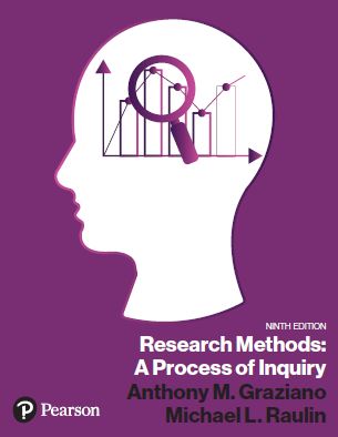
So he started with a simple difference between the Z-scores of the two variables. He squared the differences to make them all positive and divided by N. This first draft of his index of relationship is illustrated in the first equation below. It is conceptually easy to understand; it is simply the averaged squared distance between the Z-scores of the two variables.
This seems, conceptually at least, like a reasonable index of the degree of relationship between two variables. But when you first create a new index of something, you want to test it to see how it works. You could do this yourself, even with the little bit of statistics that you have already learned. Start by creating two scatter plots that represent a perfect positive and a perfect negative relationship. You just draw a straight line in a two dimensional space, place say 20 points on that straight line, and then read off the XY coordinates for each of those 20 points. Then plug those numbers into the formula above.
Now you might try two or three lines that represent perfect relationships to see if you get consistent results from your index. If you do that, you will discover that a perfect positive relationship will produce a score on this index of 0.00. The reason is that in a perfect positive relationship, the Zx and Zy value will always be the same, so the quantity Zx-Zy is always equal to zero. Give it a try and see for yourself.
What will this index show if you have a perfect negative relationship? Will the index produce a stable number that will tell us at a glance that we have a perfect negative relationship? If you try it, you will find that you get 4.00, and you will get it every time. If you are good at algebra, you can produce a mathematical proof for that outcome, but we do not need to get that sophisticated to understand this process.
So Pearson's original index produces scores from 0.00 to 4.00, with zero indicating a perfect positive relationship and 4.00 indicating a perfect negative relationship. If you create some more scatter plots, this time representing weaker relationships, you will see that the index does a beautiful job of capturing the degree of relationship. You will also find that if you choose X and Y scores completely randomly, so that there is no relationship, that you will get scores around 2.00 on this index, which is exactly half way between a perfect positive and a perfect negative relationship.
The only problem is that the numbers for this index are not intuitive. A perfect intuitive index would use the sign of the index to indicate the direction of the relationship and the size of the index to indicate the strength of the relationship.
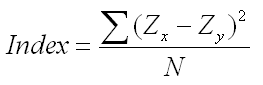
Can we convert this original index into another index with the features we just described? First we need to flip the direction of the index, because you would expect that perfect positive relationship to be indexed with a number larger than the number for the perfect negative index. We can do that by simply taking the negative value of the index (the second equation below). So now a perfect positive index is still 0.00, but a perfect negative index is -4.00.
If we move the scale over two units by adding 2, our new index will range from a -2.00 to a +2.00, representing a perfect negative and a perfect positive relationship respectively (the third equation below).
Finally, it might be convenient to have the the end points at -1.00 and +1.00, which we can easily do by multiplying the index by 1/2 (the fourth equation below). The resulting equation was the index that Pearson first proposed and called rxy.
Note that there is no sophisticated mathematics in any aspect of what we have done. We are using nothing more than high school algebra and a clever starting point to produce this index of the degree of relationship between two variables.
Pearson's index quickly caught on. With a little algebra, this time a bit more complicated, you can show that the formula above for rxy was equal to the average product of the Z-scores for the two variables, which is shown below. This is where the name product-moment correlation came from. We are using an index that is based on the product of the two scores that show how far each score is from the mean. (Statisticians call the directional distance from the mean the "moment" of the score.)

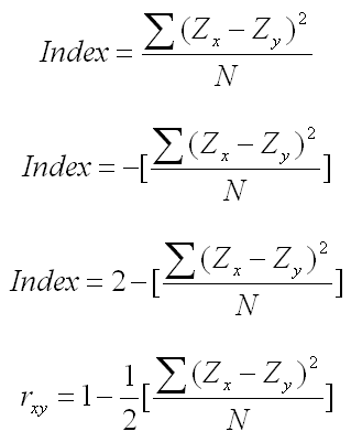
There were no computers when all of this early work was done. In fact, there were no calculators. Since Z-scores are often numbers like -1.236348, working with them is a pain. Therefore, there was a good reason to find an equation that did not produce difficult-to-work-with numbers. In fact, you will find that virtually all of the statistical procedures developed before the advent of computers have both a definitional formula, which tells you what the statistic represents conceptually, and a computational formula, which gives you an easier way to compute the statistic with nothing more than a pencil and paper.
The computational formula for the correlation is written below. It certainly does not look easier than the equation above, but if all the X and Y values are integers, all of the values in this formula will also be integers except for the correlation itself.
What is the point of this historical recreation of the development of the Pearson product-moment correlation? It is important that you realize that these are not magical procedures. Instead, they are clever ways of solving a problem.
Pearson simply wanted an index that would tell you at a glance the strength of the relationship between two variables. With a little trial and error, he found one. With a little algebra, he modified it so that its range and direction was intuitive. A little more algebra showed that the index developed one way could be expressed in an entirely different way that was shorter and more elegant. Finally, a little more algebra produced a computational formula that was much easier to use before the time of computers and electronic calculators. It is clever, and it works well, but it is not magic.
We will generally not be providing such history behind the development of statistics, but we thought it a useful lesson to know that this process is not as impossibly complex as the quick presentation of the formulas and descriptions might lead you to believe.
|
Use the Back Arrow Key on the Browser Program to Return |