 Graziano & Raulin
Research Methods (9th edition)
Planned Comparisons and Post Hoc Tests
Finding a significant F-ratio when you are comparing more than two groups only tells you that at least one of the groups is significantly different from at least one other group. To find out which groups are different from which other groups, you have to conduct additional analyses, which are referred to as probing (short for probing the results of the ANOVA).
There are two general approaches to probing the results of a significant ANOVA. The first is to decide what means should be significantly different from what other means before the study is conducted based on a theoretical analysis of the study. This approach involves performing planned comparisons. This is the preferred approach if you have a strong theoretical reason to expect a specific pattern of results.
The other approach is post hoc tests, which are not planned in advance, but rather conducted "after the fact" to see which means are different from which other means. We will cover both in this section.
Planned Comparisons
Planned comparisons also go by the name of contrasts, which technically refer to the weighted sum of means that define the planned comparison. Let's use an example to explain what that means.
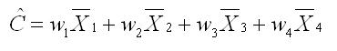
Suppose that you have four groups in your study and that one of your hypotheses is that groups 3 and 4 should differ from one another. This hypothesis, formulated before the study is ever run, is that basis for a planned comparison. To test this hypothesis, we need to set up a contrast in the following form. We will use the letter C with a caret over it to indicate our contrast. The caret simply means that our contrast is based on estimates of population means from on our samples, rather than being based on the actual population means. So the equation for the contrast in its general form (for four groups) looks like this. Each w in the equation is the weight that is multiplied by its particular mean.
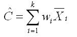
We can rewrite that equation for the contract in a more general form, as shown below. In this equation, we sum across the number of groups (k), multiplying each of the means by the appropriate weight.
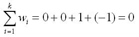
Now, how do we determine the set of appropriate weights for a given contrast. The appropriate weights are those that define the comparison that you want to make and, at the same time, sum to zero. In our example of a planned comparison, we want to compare groups 3 and 4, but we must have a weight to multiple against each of the four means. The way to exclude groups 1 and 2 from the analysis is to give both of them a weight of 0. Then if we give group 3 a weight of 1, the weight for group 4 would have to be a -1 in order for the sum of the weights to equal zero, as shown here.
Any comparison that we can specify in words can be specified with a set of weights that meet the criterion that the sum of the weights is zero. For example, if we wanted to compare the average of groups 1 and 3 against the average of groups 2 and 4, we could use the weights +1, -1, +1, and -1 for groups 1 through 4, respectively.
By the way, any set of weights that define the expected relationship and sum to zero will work for the contrast. So we could just as easily used +2, -2, +2, and -2 or -.25, +.25, -.25, and +.25. The signs can be reversed and the numbers can be any multiple or fraction of a set of weights that work. It is convenient to use simply integers, but not necessary.
We can also define other contrasts. For example, we might hypothesis that group 4 will be different from the average of groups 1 and 2. Because group 3 is excluded from this hypothesis, its weight must be zero. Groups 1 and 2 are to be averaged, so they must have the same weight. If we arbitrarily give them weights of +1 and +1, then the weight of group 4 must be -2, because that is the only weight that will produce of sum of weights that is equal to zero.
So getting back to our initial example of a planned comparison (comparing groups 3 and 4), our contrast is computed using the equation below.
![]()
To test this planned comparison, you will compute a t using the following equation.
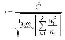
This equation looks complicated, but you are already familiar with each of the terms. The numerator is the contrast that you just computed. The denominator is a function of the Mean Square within groups MSw), which is routinely computed for the ANOVA. The denominator is also a function of the weights used in the computation of the contrast, and the sample sizes for each of the groups.
The computed value of t has to be compared with the critical value, and to determine the critical value, you must know the degrees of freedom and decide on your alpha level. The degrees of freedom is equal to N - k, which happens to be dfw. So you can get that value from the ANOVA summary table.
If you want to see how you set up a planned comparison using SPSS for Windows, click on the link below. Use the browsers back arrow key to return to this page.
| Compute a Planned Comparison using SPSS |
| USE THE BROWSER'S BACK ARROW KEY TO RETURN |
Multiple Planned Comparisons
You need not restrict yourself to a single planned comparison, but there is a requirement that all planned comparisons be independent of one another. Independence in this case is defined statistically. If two comparisons are independent, the product of the weights for the two contrasts, summed across the groups, is equal to zero, as shown in the equation below.

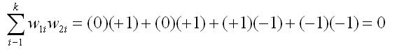
This principle of independence is best illustrated with a couple of examples. Our initial example of a planned comparison used the following weights: 0, 0, +1, and -1. Suppose we wanted to test a second planned comparison that said that the average of groups 1 and 2 is different from the average of groups 3 and 4. Would this second planned comparison be independent of the first planned comparison?
To test the second planned comparison, we might use weights of +1, +1, -1, and -1, although you learned that this set is one of many possible sets that would test this hypothesis. So are these two planned comparisons independent of one another. Plugging the values into the equation above, we get the following.
Now lets suppose that we are considering testing a third planned comparison that the average of groups 1 through 3 is different from group 4. A set of weights that would test this hypothesis is +1, +1, +1, and -3. Is this planned comparison independent of both the first and second planned comparisons. The two equations below will check on independence.
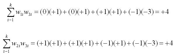
The sum of the product of the weights for the two planned comparisons in both cases is not equal to zero. So the third planned comparison is not independent of either the first or the second. Both the first and second planned comparisons in our example can be tested, because they are independent, but if we test either of those, we cannot test the third proposed planned comparison.
Because any set of planned comparisons must be independent of one another to be statistically appropriate, it is a good idea to plan those comparisons carefully before collecting any data. Good researchers will list all of the planned comparisons that seem theoretically reasonable and then check to see which ones are independent of one another. Armed with that information, they select the planned comparisons that are most theoretically important and also independent of all the other planned comparisons they intend to run. If your research is guided by a clear theory of what to expect, you will find that the theory guides you just as clearly about which planned comparisons are most important to testing the theory.
Post Hoc Tests
Post hoc tests are typically used to evaluate pairs of groups to see if they are statistically significant from one another. Unlike planned comparisons, these evaluations are not planned in advance, but rather represent a search "after the fact" to see where the statistically significant differences exist.
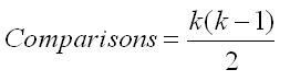
The number of such comparisons that can be done following a one-way ANOVA depends on the number of groups. There is a simple formula for computing the number of possible comparisons, which is shown below. The letter k in the formula is the number of groups. So, if you have 4 groups, you have 6 possible comparisons (4*3/2). If you have 8 groups, you have 28 possible comparisons (8*7/2). Clearly, the number of possible 2-group comparisons increases rapidly as the number of groups increases.
One of the problems with conducting so many comparisons is that you increase the probability of finding some of the differences statistically significant by chance alone. Statisticians refer to this problem as inflating the Type I error level. Remember that Type I errors are rejecting the null hypothesis when the null hypothesis is true. In other words, a Type I error is concluding that the evidence suggests that the populations differ when in fact they do not differ.
We set the level of Type I error when we set the alpha level. So if alpha is set at .05, it means that we will make a Type I error 5% of the time. But that means that if you do 20 comparisons, you can expect one of them to be significant by chance alone, and you will have no way of knowing which of the significant differences you find represent that Type I error. Statisticians address this problem in post hoc testing, when it is common to have multiple comparisons, by making the criteria for significant more stringent. Post hoc tests build this additional stringency into the procedures. That is why is is absolutely inappropriate to use a standard t-test as a post hoc test.
There are more than a dozen post hoc tests that have been published. Going over all of them is beyond the scope of this text. Instead, we will introduce you to to the names of some of the more popular tests and describe how they compare to one another.
The post hoc tests fall into two broad class: tests that do and do not assume homogeneity of variance. Homogeneity of variance means that the variances are statistically equal in the groups, which means that the differences in variances found are small enough to be due to sampling error alone.
Tests that Assume Homogeneity of Variance. The largest class of post hoc tests assumes that we have homogeneity of variance. The most frequently used tests in this category are the Tukey test (sometimes called Tukey's Honestly Significant Difference test or HSD), the Scheffe test, the Least Squared Difference test (LSD), and the Bonferroni test.
All of these tests are variations on a t-test, in which some specific steps are taken to control for the problem of inflating the level of Type I error by doing so many multiple comparisons. The Bonferroni test does this in the most explicit manner, essentially using a standard t-test, but computing the critical value of t that will produce what is called an experiment-wise alpha of a given level. An experiment-wise alpha of .05 means that the probability of making a Type I error anywhere in the experiment is set at .05. The only way you can do that if you have multiple comparisons is to use a more stringent alpha level for each of those comparisons. Exactly how stringent will depend on how many comparisons you are making. The more comparisons you make, the more stringent your alpha must be for each of them in order to control the experiment-wise alpha level.
The other tests mentioned here, as well as half a dozen other published post hoc tests, each take a different approach to controlling the experiment-wise level of Type I error. The reason that so many post hoc tests exist is that there is no agreement on which test achieves this goal best.
We can roughly rank order the tests on how conservative they are, meaning how strong the evidence must be before they declare a given comparison significant. However, there is considerable debate about whether a given test is either too conservative or not conservative enough. That is why most computer analysis programs will give users a dozen or more choices for post hoc tests. Each researcher tends to have his or her preferred post hoc test.
Tests that Do Not Assume Homogeneity of Variance. If you do not have homogeneity of variance, any statistical procedure that implicitly assume homogeneity will be distorted by the violation of this assumption. More importantly, the distortion will be in the direction of suggesting a difference exists when in fact it does not exist. In other words, the violation of this assumption increases the level of Type I error. Remember that we set the level of Type I error (called alpha) low, because we want to avoid these kinds of errors. So, from a statistical perspective, we have a serious problem.
There are several post hoc tests, the best known of which is Dunnett's C test, that correct for the problem of not having homogeneity of variance. These tests all tend to be more conservative than the tests that assume homogeneity, but they also tend to be more accurate if the variances in the groups actually do differ.
If you want to see how you set up a post hoc tests using SPSS for Windows, click on the link below. Use the browsers back arrow key to return to this page.
| Compute Post Hoc Tests using SPSS |
| USE THE BROWSER'S BACK ARROW KEY TO RETURN |