Relative Scores

In this section, we will use some of the statistical information that you have already learned to solve the practical problem of how to indicate the relative standing of a person on a measure.

As part of this section, you will learn about the standard normal distribution, which is a distribution that is defined by a mathematical equation. Such mathematical distributions are a critical part of the inferential statistical process that we will be covering later.

Percentile Ranks

Relative scores indicate where a person stands within a specified normative sample. In general, scores have little meaning unless you know how other people scored. For example, on probably most of the exams that you have taken in school, you need to be correct 70% or more of the time just to pass the course, yet the standardized tests that you took as part of the college admission process are designed so that less than half of the people taking them get 70% or more of the questions correct.

To know how good a score is, you need to know what other people got. For example, a professional baseball player who got a hit only half the times he went up to bat would be by far the greatest hitter of all time. Most professional baseball players only get a hit about every fourth time at bat. In contrast, a driver who only reached his or her destination without an accident half the time would be considered so bad that no insurance company would cover the person. Most people arrive safely at their destination 99+% of the time.

We are constantly seeking information about relative scores, sometime even before the scores have been computed. How many times have you walked out of a test and asked other students whether the test seemed hard or easy. If you thought it was hard, and therefore are worried that you did not do well, you are likely to feel a little better after other students tell you that it seemed very hard to them as well.

The most basic relative score is the percentile rank, which specifies the percentage of people in the normative group who score lower on the measure than yourself. So if you scored at the 25th percentile, it means that 25% of the people score lower than you and 75% score higher than you. Percentile ranks can range from 0 (for the person with the lowest score) to 100 (for the person with the highest score).

Most often percentile ranks are computed from a frequency distribution. Let's again use the frequency distribution that we have used before for examples. That distribution is below. Suppose that we want to compute the percentile rank for a score of 15. From the table, we can see that there are 333 people with a score below 15, but what do we do with the 33 people who have exactly 15? Do we count them as scoring above or below our person with a score of 15. The tradition is to assume that half of the people with the same score are below and half are above. That means that we have 33/2=16.5 with a 15 that we consider to be lower than us, and the same number with a score of 15 that we consider to have a score higher than us. We add the 16.5 people to the 333 people with lower scores of 14 or lower to get the number of people with scores lower than ours.

Score	Frequency	Cumulative Frequency
17	8	394
16	20	386
15	33	366
14	48	333
13	71	285
12	85	214
11	58	129
10	39	71
9	21	32
8	11	11

There are a total of 394 people. To get the percentile rank, we divide the number of people below our score by the total number of people and multiply by 100 (to convert the proportion to a percent). In this case, the percentile rank is 89 [(349.5/394)*100].

We traditionally round percentile ranks to two significant digits. So we rounded 88.705584% to 89%.

Standard Normal Distribution

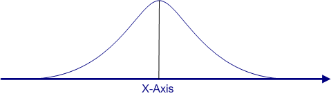
Many variables in psychology tend to show a distinctive shape when graphed using a histogram or frequency polygon. The shape resembles a bell shaped curve like the one shown below. This classic bell shaped curve is called a normal curve or normal distribution.

The normal curve is perfectly symmetric. The right half and left half are mirror images of one another. The curve also does not quite reaches zero, although it gets very close. The shape of the normal curve is actually determined by a complex equation, with dictates the height of the curve at every point. You need not know the details of this equation, but you should know that the equation includes two variables. They are the mean and the standard deviation. The mean dictates where the middle of the distribution is, which is the highest point of the curve and the point that separates the the area under the curve into two equal segments. The standard deviation determines how spread out the curve is.

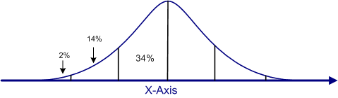
Because the normal curve is based on an equation, it is possible to know exactly how high the curve is at every point and how much area is under the curve between any two scores on the X-axis. The figure below marks off 1 and 2 standard deviations both above and below the mean. The area under the curve between the mean and one standard deviation below the mean is approximately 34%, as shown in the figure. More precisely, it is 34.13%. We will show you where that number comes from shortly.

Because the curve is symmetric, the area between the mean and one standard deviation above the mean is also 34%. Similarly, the area between 1 and 2 standard deviations, either above or below the mean, is approximately 14%, and the area beyond 2 standard deviations is 2% on either side of the distribution. All of these areas are determined by the equation for the normal curve, but you do not need to use this equation, because the values are computed for you and available in a table called the Area under the Standard Normal Curve Table. If you click on the link to this table, you can see what it looks like.

To use the Standard Normal Table, you need to know a little more about the normal curve and you need to learn about the standard score, also known as the Z-score.

If you look at the two normal curves above, you might recognize that there are no scores listed on the X-axis. Remember that the location on the X-axis is determined by the mean of the distribution and the spread of the curve is determined by the standard deviation of the distribution. But you can convert a normal curve with any mean and variance into a standard normal distribution, which is a a normal curve with a mean of zero and a standard deviation of 1.

If the curve above were a standard normal distribution, the labels on the X-axis at the lines that divide the curve into sections would be -2, -1, 0, +1, +2, read from left to right. The table we showed you earlier gives the areas under the curve of such a standard normal distribution.

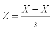
Shown below is the equation that converts any score to a standard score using the values of the score and the mean and standard deviation of the distribution. A standard score shows where the person scores in a standard normal distribution. It tells you instantly whether the score is above or below the mean by the sign of the Z-score. If the Z-score is positive, the person scored above the mean; if it is negative, the person scored below the mean. The size of the Z-score indicates how far away from the mean the person scored.

If you want to see exactly how the standard normal distribution and the Z-score can be used to compute a percentile rank, you can click on this link. Besides walking you through the process, this link provides exercises to help you master this concept and procedure.

Other Relative Scores

The score on any measure could be converted to a Z-score, which would tell you at a glance how a person scored relative to the reference group. For example, if someone tells you that her Z-score on the exam was +1.55, you know immediately that she scored above the mean and enough above the mean that she is near the top of the class. Remember, most of the normal distribution is contained between the boundaries of -2.0 and +2.0 standard deviations. There is only about 2% of the area under the curve in each of the tails. If another student tells you the his exam score was a Z of -.36, you know that he scores a bit below the mean.

With the standard normal table, you could compute the percentile rank for each of these students in a few minutes. Of course, this procedure is only legitimate if the shape of the distribution of scores is normal or very close to normal. If the shape is not normal, the Standard Normal Table will not give accurate information about how the proportion of people who score above and below a given score.

Although Z-scores are very useful and allow people to judge the relative performance of an individual quickly, many people get easily confused by the negative numbers that are possible with Z-scores. Consequently, many tests compute Z-scores, but then translate them mathematically to avoid negative numbers.

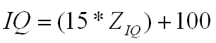
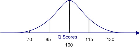
For example, the IQ test produces a distribution of scores that is very close to normal. However, the IQ test does not give a person's score as a Z-score; instead, the IQ test reports the score as an IQ score. The IQ score is simply the Z-score multiplied by 15 and then added to 100, as shown in the equation below. The values of 15 and 100 are arbitrary, but the effect of this transformation is to produce a normal distribution with a mean of 100 and a standard deviation of 15. So the IQ distribution looks like the figure below. Note that this figure is identical in shape to all the other figures in this section. The only difference is that the scores on the X-axis are IQ scores. So just over 95% of people have IQ scores between 70 and 130, and no one has a negative IQ.

Standardized tests often perform a similar transformation to avoid negative scores. For example, the Scholastic Aptitude Test (SAT) used for college admission and the Graduate Record Exam (GRE) used for admission to graduate school are both standardized so the the mean of the subtests is 500, with a standard deviation of 100. So if you score 450 on the verbal section of the SAT, you are scoring .5 standard deviations below the mean, which puts you at the 31st percentile. (See if you can do the computations and use the standard normal table to verify this percentile rank. This link shows you the method to make this computation.)

The Normative Sample

Z-scores and transformed Z-scores, such as SAT scores, are very handy and are used extensively in reporting test scores. But it is critical to understand that the score is meaningful ONLY if you take into account the normative sample.

A quick example will illustrate this point. Let's assume that Dan took the SAT as a High School senior and scored 650 on each subtest. That is 150 points above the mean (1.5 standard deviations) and would place him at approximately the 93rd percentile.

Four years later, after doing well in college, he decides to go to graduate school, and so he takes the GRE. This time he only obtained a 550 on each of the subtests. What happened? Why did his performance decrease despite the fact that he worked hard in college and did very well?

You may already have guessed the answer to that question. In effect, we are trying to compare apples and oranges. The scores on the SAT and the GRE mean entirely different things, because they are based on entirely different normative samples.

The SAT is taken by people who expect to complete high school and are considering going on to college. In contrast, the GRE is taken by people who expect to graduate from college and plan to go onto graduate school. Anyone who drops out of college or does poorly in college is unlikely to take the GRE. In other words, the normative sample for the GRE is much more exclusive than for the SAT. Dan's GRE score would place him in the 70th percentile of the people applying for graduate school, who are a pretty elite group academically. Most of the people who took the SAT did not take the GRE, and most of the people who take the GRE did very well on the SAT. The competition (i.e., the normative group) was tougher for the GRE than the SAT.

Whenever you are given a normative score, such as a Z-score, percentile rank, or score on a standardized test, you should always consider the nature of the normative sample. A person making $500,000 per year may be one of the best paid people in the country (the normative sample including all workers), but one of the lowest paid CEOs for a Fortune 500 company (a different normative sample).

Go to the Next Page