Sampling Distributions

You were introduced to the standard normal distribution in the section on relative scores. In this section, you will learn how to use the concepts of probability to compute percentile ranks using the standard normal distribution. You will also learn about the concept of sampling distributions, the variables that affect them, and how to use them. This section will give you the last of the tools that you need to understand inferential statistics.

Using the Standard Normal Table

As you learned earlier, the normal curve is determined by a mathematical equation, and any normal distribution can be converted to a standard normal distribution by subtracting the mean from each score and dividing by the standard deviation. This transformation turned each score into a standard score or Z-score. In this section we will see how the concept of probability can be applied to the standard normal distribution and, by extension, to any distribution.

To review, the standard normal curve has a mean of zero and a standard deviation of 1. The distances between the mean and any point on the standard normal curve can be computed mathematically. In fact, the computations have already been done and are tabled in something called the standard normal table.

Shown below is a small part of the standard normal table, which is divided into three sets of three columns. In the columns labeled (a) are the Z-scores. The standard normal table included on this website has every Z-score from 0 to 3.25 in .01 increments, and from 3.25 to 4.00 in .05 increments. This is normally more than enough detail for solving the typical problems using this table.

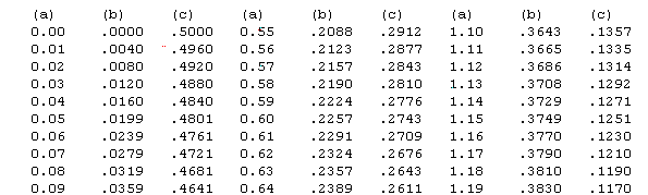
The columns labeled (b) show the area under the curve from the mean to that Z-score, and the columns labeled (c) show the area from that Z-score to to end of the distribution. For example, find the Z-score of .60 in the abbreviated table below. Note that the area from the mean to that Z-score is .2257 and the area from that Z-score to the end of the tail is .2776. These two numbers will always add to .5000, because exactly 50% (a proportion of .5000) of the curve falls above the mean and 50% below the mean in a normal curve.

The figure below illustrates this Z-score and the areas that we read from the table.

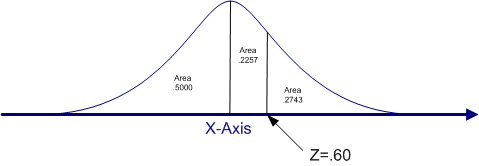
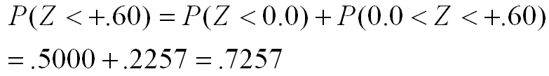
How can we use this information to determine the percentile rank for the person whose Z-score is .60? Remember that the percentile rank is the percent of individuals who score below a given score. If you look at the figure above, you will see that the area below the mean is .5000 and the area between the mean and a Z-score of .60 is an additional .2257. Therefore, the total area under the standard normal curve that falls below a Z of .60 is equal to .5000 plus .2257, which is .7257.

We are essentially using the addition rule of probability in that we are computing the probability of getting a Z-score of +.60 or lower as the probability of getting a Z-score below 0 plus the probability of getting a Z-score between 0 and +.60, as shown below. The value of .7257 is a proportion. The total area under the curve is 1.00 expressed as a proportion and 100% expressed as a percent. To convert a proportion to a percent, you multiply by 100, which is the same as moving the decimal point to the right two places. Therefore, the proportion of .7257 becomes a 72.57%. This approach can be used with any Z-score to compute the percentile associated with that Z-score.

Let's work another example, this time with a negative Z-score. What is the percentile rank for a Z-score of a -1.15.

The first step is to always draw the picture. Quickly sketch a normal curve and place the score in approximately the right space. Remember, the sketch of a normal curve stretches a bit more than two standard deviations above and below the mean, so a Z-score of -1.15 will be about half way between the mean and the end of the lower tail, as shown in the figure below. (Technically, the normal curve stretches from a minus infinity to a plus infinity, never quite touching the X-axis. However, virtually the entire area of the curve is in the section from a Z = -2.00 to a Z = +2.00.)

Again, we can use the abbreviated standard normal table above to determine the areas of that section of the curve.

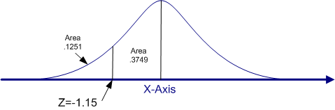
The most common mistake made by students with negative Z-scores is to assume that the area listed in column (b) of the standard normal table is the area below the Z-score. It is always the area between the mean and the Z-score. It is the area below the Z-score down to the mean for positive Z-scores, but it is an area above the Z-score up to the mean for negative Z-scores.

Again, if you draw the picture and carefully interpret the meaning of the standard normal curve, you can avoid these common mistakes. In this case, the area under the curve and below a Z-score of -1.15 is .1251. Therefore, the percentile rank for this score is 12.51%. Just over 12% of the sample scored lower than this score.

Sampling Distributions

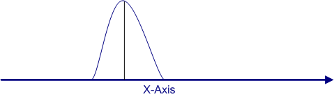
Let's assume for the sake of argument that we have a large population, say a million people, and that we have scores on all of the people in that population. It is unlikely that we really would have scores on everyone in a population that large, but for the sake of argument, we will say that we do. Furthermore, we have graphed the distribution for that population and found that it has a moderate positive skew, as shown in the curve below.

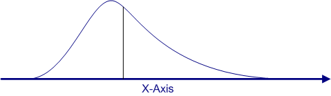
The mean for this population is shown with a vertical line. Because the distribution is skewed, the mean is pulled a bit from the peak of the distribution. If we take a random sample of 100 people from that population and produce a frequency polygon for the sample, we will get a graph that resembles this curve. With just 100 people, the graph will not be as smooth, but you will probably be able to tell by looking at the graph that there is a slight positive skew.

If you take a bigger sample, say 500 people, the resulting graph will be very similar in shape to the population distribution shown here. The reason is that random samples tend to produce representative samples, so the range and distribution of the scores in a distribution drawn randomly from a population should provide a reasonably accurate representation of the shape of the distribution. The larger the sample size, generally the more likely that the sample will resemble the distribution of the population.

This is the first concept to remember about sampling: The larger the sample, the more likely that the sample will accurately represent the population, provided that the sample is unbiased. A random sample is the best way to produce an unbiased sample.

We can think of a sample of 500 people that we select from the population as if it were 500 samples of size N=1. In other words, we are drawing 500 individual samples of one person. The mean for a sample of one person is the score for that person, because there is only 1 score to sum and we are dividing by N, which is equal to 1.

If we think of the distribution not as a distribution of scores, but as a distribution of means from multiple samples of just one person, the distribution becomes a sampling distribution of the mean. Technically, a sampling distribution of the means is a theoretical concept, which is based on having all possible samples of a given sample size. But if we had 500 samples, we could get a pretty good idea what the distribution would look like. A sampling distribution of means is an important concept in statistics, because all inferential statistics is based on the concept.

If our samples only contain one person, they may each provide an unbiased estimate of the population mean, and the one person could be drawn from anywhere in the distribution. But what if we draw 500 samples of two people, compute the mean for each sample, and then graph the results. This would be a sampling distribution of the means for samples of size N=2. What do you think will happen?

Suppose in the first sample, we happen to draw a person who scored in the tail as our first participant. What will the second participant look like? Remember that in random sampling, the selection of any one person does not affect the selection of any other person, so the initial selection will not influence the selection of the second person in the sample, but on average, it is unlikely that we would sample two people that are both in one tail of the distribution. If one is in the tail and the other is near the middle of the distribution, the mean will be halfway between the two.

What will happen is that the distribution of means for a sample size of 2 will be a little less variable than for a sample size of 1. This is our second concept about sampling: A larger sample size will tend to give a better (i.e., more accurate) estimate of the population mean than a smaller sample size.

For the sake of illustration, we have graphed the likely distribution of means for 500 samples of size N=2 below.

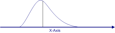
Note how the sampling distribution of the means for a sample size of 2 is somewhat narrower and a little less skewed than for a sample size of 1. The mean of this distribution of means is still the population mean, so that value has not shifted. You can see that the skew has decreased a bit in two ways. The first is that the tail to the right of the distribution is not quite as long. The second is that the mean is now closer to the peak of the distribution.

What would happen if our sample size were larger still? Let's assume that we take 500 samples of 10 people each, computer their mean, and then graph those means to see what the distribution looks like. The figure below is what you can expect to find.

Again, the mean of this distribution of means has not shifted, because the mean of a sample is an unbiased estimate of the population mean. What that means is that if we took all possible samples of a given sample size and computed the mean for each sample, and then we computed the mean of all those means, the result would be the population mean.

That is quite a mouthful to say and most students have to read that last sentence two or three times to let the idea settle in. This is a theoretical concept, although it can be proved mathematically. However, in practice, it is pretty close to impossible to actually achieve the goal of identifying every possible sample of a given size. Nevertheless, it is possible to predict exactly what will happen with this sampling distribution of the mean for any sample size.

As the sample size increases, two things will occur. First the variability of the sampling distribution of means will get smaller as the sample size increases. This is just another way of saying that the estimate of the population mean tends to be more accurate (that is, closer to the population mean) as the sample increases. Therefore, the means for larger samples cluster more tightly around the population mean.

The second thing that happens is that the shape of the distribution of means gets closer to a normal distribution as the sample size increases, regardless of the shape of the distribution of scores in the population. If you look at the three graphs above (samples sizes of 1, 2, and 10, respectively), we went from a moderate and clearly visible skew to a barely noticeable skew by the time we reached a sample size of 10. With a sample size of 25 or 30, it would be virtually impossible to detect the skew.

This movement toward a normal distribution of the means as the sample size increases will always occur. Mathematicians have actually proved this principle in something called the central limit theorem. For all practical purposes, the distribution of means will be so close to normal by the time the sample size reaches 30, that we can treat the sampling distribution of means as if it were normal.

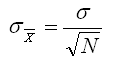
Mathematicians have also determined what the theoretical variability of a distribution of means should be for any given sample size. If we knew the population standard deviation, we could easily compute the standard deviation for the theoretical distribution of means using the following formula. The only new terminology in this equation is that we have subscripted the population standard deviation symbol with the symbol for a mean to indicate that, instead of talking about the standard deviation of a distribution of scores, we are talking about the standard deviation of a theoretical distribution of means. This standard deviation is referred to as the standard error of the mean (sometimes just called standard error), although it would be just as legitimate to call it the standard deviation of the means, because that is what it is.

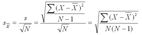
Of course, we do not know population parameters like the standard deviation. The best we can do is to estimate the population standard deviation with the standard deviation from our sample. Remember that the formula for the standard deviation had be be corrected to avoid producing a biased estimate of the population standard deviation. It is this unbiased estimate formula that should be used when we compute the standard error of the mean.

The equation below includes three forms. The first indicates the definition, which is identical to the above equation. In the second form, we have substituted the formula for the unbiased estimate of the population standard deviation for s in the numerator. The third form was simplified from the second form with a little algebra.

Confidence Intervals

Once again, we can now pull together several separate concepts and create a new statistical procedure that you can use, this time called the confidence interval.

If we draw a single sample of participants from a population and compute the mean for that sample, we are essentially estimating the mean for the population. We would like to know how close our estimate of that population mean really is.

There is, unfortunately, no way of knowing the answer to that question from just a single sample, but we can approach the question in a different way. Instead of simply saying that the sample mean is our best estimate of the population mean, we can give people an idea of how good an estimate it is by computing a confidence interval.

A confidence interval is a range of scores in which we can predict that the mean falls a given percentage of the time. For example, a 95% confidence interval is a range in which we expect the population mean to fall 95% of the time. How wide or narrow that interval of scores is will give people an objective indication of how precise our estimate of the population is.

Now remember the principle that you learned earlier that the larger the sample size, assuming the sample is unbiased, the more precise your estimate of the population mean. That suggests that with larger sample sizes, we can have a narrower confidence interval, because our mean from a large sample is likely to be close to the population mean.

The secret to creating the confidence interval is to know not only the mean and standard deviation of your sample, but also the shape of the distribution. If we are talking about a confidence interval about a mean, our distribution is the sampling distribution of the means, and the central limit theorem tells us that is will be normal in shape if the sample size is reasonably large (say 30 or more). So we can use the standard normal table and a relatively simple formula to compute our confidence interval.

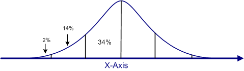
When we introduced the normal curve earlier, we noted that the the distance from the mean almost to the end of the tail was two standard deviations, and that there was about 2% of the area under the curve that was beyond two standard deviations in each tail. If we want to do a 95% confidence interval, we want to know the exact value that will cut off 2.5% in each tail (a total of 5%). Remember that the figures are listed as proportions in the standard normal table, so 2.5% is .0250 in the tail. Click on the link to that table and look up the Z-score that cuts off the last 2.5%, and then return to this page with the back arrow key.

Did you find that a Z of 1.96 cuts off the 2.5% in the tail?

You now have all of the elements that you need to do a confidence interval for the mean (your sample mean and standard deviation and this cutoff point in the normal curve. So let's set up the logic and then introduce you to the formulas. Focus on the logic, because you can always look up the formulas when you need them.

If we have a reasonable large sample, with its associated sample mean, standard deviation, and sample size, we have the ingredients for not only estimating the population mean, but also estimating how close our estimate is likely to be. The steps and logic are as follows:

Our sample mean is our best estimate of the population mean, because we know it is an unbiased estimate. Therefore, any confidence interval we create will be around that estimate.
Even though we have only taken one sample, we know the equations that will predict the standard deviation of a distribution of means of that sample size (our standard error of the mean). We simply divide our unbiased estimate of the population standard deviation by the square root of our sample size.
Even though we only took one sample, we know from the Central Limit Theorem that the distribution of means would be normal for large samples sizes. Therefore, we can use the standard normal table to know how far above and below our sample mean we must go to be confident that the population mean is within the range. We just determined that a 95% confidence interval stretched from 1.96 standard deviation units below the mean to 1.96 standard deviation units above the mean.
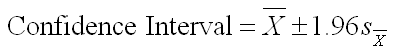
With these elements, we can use the following formula to compute the lower and upper limits of the confidence interval using the following equation. The equation reads the sample mean plus or minus 1.96 standard error of the mean units. The most common mistake made by students here is not recognizing that we are using the standard error (the standard deviation of the theoretical distribution of means) and NOT the standard deviation of the sample.

The easiest way to understand this process is to work through an example. Let's assume that we have sampled 100 people and computed the sample mean as 104.37 and the sample standard deviation as 14.59.

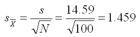
We used the formula for the standard deviation that gives us an unbiased estimate of the population value. In fact, from now on, we will only be using that formula (the one in which we divide by the square root of N-1). We can use this information to compute the standard error of the means, using the formula below.

Now before we plug the numbers into the confidence interval formula, let's first draw the figure to show what we are doing. We know that the sampling distribution of the means will be normal and will have an estimated mean of 104.37 and an estimated standard error (the standard deviation of that distribution of means) of 1.459, which we just calculated. So our confidence interval will look like the following.

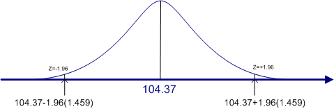
This figure shows the theoretical distribution of the means for a sample of size 100, based on the mean and standard deviation from that sample. Again, our sample mean is our best estimate, but the population mean may be a little lower or higher than this particular sample mean. However, we now have a way to say just how much lower or higher it is likely to be.

The lower limit is 104.37-1.96(1.459), which equals 101.51 (rounding to two decimal points). The upper limit is 104.37+1.96(1.459), which equals 107.23. Therefore we can say that we are 95% confident that the population means lies between 101.51 and 107.23.

Go to the Next Page