Linear Regression

As you learned in Chapters 5 and 7 of the text, the value of correlations is that they can be used to predict one variable from another variable. This process is called linear regression or simply regression. It involves fitting mathematically a straight line to the data from a scatter plot.

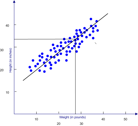
Below is a scatter plot from our discussion of correlations. We have added a regression line to that scatter plot to illustrate how regression works. We compute the regression line with formulas that we will present to you shortly. The regression line is based on our data. Once we have the regression line, we can then use it to predict Y from knowing X.

The scatter plot below shows the relationship of height and weight in young children (birth to three years old). The line that runs through the data points is called the regression line. It is determined by an equation, which we will discuss shortly. If we know the value of X (in this case, weight) and we want to predict Y from X, we draw a line straight up from our value of X until it intersects the regression line, and then we draw a line that is parallel to the X-axis over to the Y-axis. We then read from the Y-axis our predicted value for Y (in this case, height).

In order to fit a line mathematically, there must be some stated mathematical criteria for what constitutes a good fit. In the case of linear regression, that mathematical criteria is called least squares criteria, which is shorthand for the line being positioned so that the sum of the squared distances from the score to the predicted score is as small as it can be.

If you are predicting Y, you will compute a regression line that minimized the sum of the (Y-Y')². Traditionally, a predicted score is referred to by using the letter of the score and adding a single quotation after it (Y' is read Y prime or Y predicted).

To illustrate this concept, we removed most of the clutter of data points from the above scatter plot and showed the distances that are involved in the least squares criteria. Note that it is the vertical distance from the point to the prediction line--that is, the difference from the predicted Y (along the regression line) and the actual Y (represented by the data point). A common misconception is that you measure the shortest distance to the line, which will be a line to the point that is at right angles to the regression line.

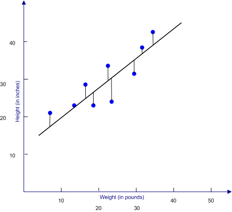
It may not be immediately obvious, but if you were trying to predict X from Y, you would be minimizing the sum of the squared distances (X-X'). That means that the regression line for predicting Y from X may not be the same as the regression line for predicting X from Y. In fact, it is rare that they are exactly the same.

The first equation below is the basic form of the regression line. It is simply the equation for a straight line, which you probably learned in high school math. The two new notational items are b_yx and a_yx which are the slope and the intercept of the regression line for predicting Y from X. The slope is how much the Y scores increase per unit of X score increase. The slope in the figure above is approximately .80. For every 10 units movement along the line on the X axis, the Y axis moves about 8 units. The intercept is the point at which the line crosses the Y axis (i.e., the point at which X is equal to zero.

The equations for computing the slope and intercept of the line are listed as the second and third equations, respectively. If you want to predict X from Y, simply replace all the Xs with Ys and the Ys with Xs in the equations below.

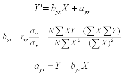
A careful inspection of these equations will reveal a couple of important ideas. First, if you look at the first version of the equation for the slope (the one using the correlation and the population variances), you will see that the slope is equal to the correlation if the population variances are equal. That would be true either for predicting X from Y or Y from X. What is less clear, but is also true, is that the regression lines for predicting X or predicting Y will be identical if the population variances are equal. That is the ONLY situation in which the regression lines are the same.

Second, if the correlation is zero (i.e., no relationship between X and Y), then the slope will be zero (look at the first part of the second equation). If you are predicting Y from X, your regression line will be horizontal, and if you are predicting X from Y, your regression line will be vertical. Furthermore, if you look at the third equation, you will see that the horizontal line for predicting Y will be at the mean of Y and the vertical line for predicting X will be at the mean of X.

Think about that for a minute. If X and Y are uncorrelated and you are trying to predict Y, the best prediction that you can make is the mean of Y. If you have no useful information about a variable and are asked to predict the score of a given individual, your best bet is to predict the mean. To the extent that the variables are correlated, you can make a better prediction by using the information from the correlated variable and the regression equation.

You can see how to compute the regression equation using SPSS for Windows by clicking one of the button below. Use the browser's back arrow key to return to this page.

Compute regression using SPSS

USE THE BROWSER'S
BACK ARROW KEY TO RETURN

Go to the Next Page