Measures of Central Tendency
Measures of central tendency indicate the typical or average score in a distribution of scores. This section covers three measures of central tendency: the mean, median, and mode.
The Mean
The mean is the arithmetic average of the scores. It is computed by adding all the scores and dividing by the total number of scores. Remember from our section on notation, we use summation notation to indicated that we should add all the scores, and we use the uppercase letter N to indicate the total number of scores. The notation for the mean of the X scores is an uppercase X with a bar across the top. Therefore the formula for computing the mean is written as follows:
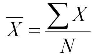
If you have several groups in your research study, it is traditional to compute the mean for each group. In such a situation, you would use a subscript notation to indicate the groups. In formulas, the groups are numbered from 1 to k. Remember that k is the letter that we use to indicate the number of groups. So using this notation, the mean for Group 1 would use the following formula.
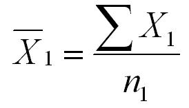
Note that we use a subscript 1 to indicate that we are computing the mean for Group 1. We are adding all the scores in Group 1 (the X1s) and dividing the the number of scores in Group 1 (n1). We use a lowercase n here, because we are NOT talking about the total number of scores in the study, but rather the number of scores in just one group of the study.
These notation rules can be a pain to learn initially, but once you get them down, you can quickly translate almost any formula into the computational steps that are required.
Although it is convenient to number groups for formulas, and we will generally be numbering groups in all of the formulas that we use, it is easier to use subscripts in your computations that are not a code. For example, if you are studying gender differences on a variable, you might compute the mean of that variable for men and women separately. Instead of using the subscripts 1 and 2 and remembering which refers to males and which refers to females, you might as well use a descriptive subscript. For example, the mean of the females might be written as follows:

Elsewhere on this website are instructions on how to compute the mean either by hand or using SPSS for Windows. To see those instructions, you click on one of the buttons below. To return to this page after viewing that material, you click on the back arrow key of the web browser that you are using to view this website.
|
Compute the mean by hand |
|
Compute the mean using SPSS |
|
USE THE BROWSER'S |
The mean is the most widely used measures of central tendency, because it is the measure of central tendency that is most often used in inferential statistics. However, as you will see at the end of this section, the mean does not always provide the best indication of the typical score in a distribution.
The Median
The median is the middle score in a distribution. It is also the score at the 50 percentile, which means that 50% of the scores are lower and 50% are higher. In the textbook, we showed how to compute the median with a small number of scores. In such a case, you:
-
Order the scores from lowest to highest and count the number of scores (N).
-
If the number of scores is odd, you add 1 to N and divide by 2 to get the middle score [(N+1)/2]. For example, if you have 15 scores, the middle score is the 8th score [(15+1)/2=8]. There will be seven scores above the 8th score and seven below it.
-
If the number of scores is even, there will be no middle score. Instead there will be two scores that straddle the middle. For example, if there are 14 scores, the 7th and 8th scores in your ordered list will straddle the middle. You can figure out which scores to focus on by dividing N by 2 and taking that score from the bottom and the one above it [e.g., 14/2=7, so you take the 7th and 8th scores from the bottom]. The median is between these two scores, so you average them. If the 7th score is 36 and the 8th score is 39, you sum the two and divide by two to get the average [e.g., (36+39)/2=37.5].
This formula works fine when there is a small number of scores and little duplication of scores, but it is not considered accurate enough when there are a large number of scores and many scores are duplicated. In such a situation, a more complicated formula is used. This formula is listed below. Don't panic; it is easier to use than it looks.

To compute a median using this formula, you must first create a frequency or grouped frequency distribution. We will use the frequency distribution that we created in the section on organizing data. That distribution is listed below.
| Score | Frequency | Cumulative Frequency |
| 17 | 8 | 394 |
| 16 | 20 | 386 |
| 15 | 33 | 366 |
| 14 | 48 | 333 |
| 13 | 71 | 285 |
| 12 | 85 | 214 |
| 11 | 58 | 129 |
| 10 | 39 | 71 |
| 9 | 21 | 32 |
| 8 | 11 | 11 |
Now we need to define each of the terms in the formula for the median. We must do this in steps. We start by finding the middle score.
- The middle score (nmedian) is the total number of scores divided by 2. In a frequency distribution that also includes a cumulative frequency column, you can read the total number of scores (N) as the number at the top of the cumulative frequency column. In this case, N is 394, so nmedian is 394/2=197.
- Next you find the interval that includes the 197th score from the bottom. To do this, start at the bottom of the cumulative frequency column and move up until you find the first number that is either equal to 197 or greater than 197. In this case, it is the interval for the score of 12. You may be surprised that we are calling that an interval, because we have only one score, but for the purposes of this computation it is an interval from 11.5 to 12.5. This is illustrated by the figure below.
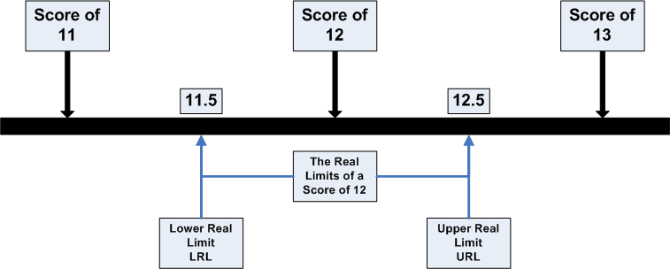
- Now we can identify all of the numbers that will go into the formula for the median. LRL stands for Lower Real Limit of the interval that contains the median. In this case, it is 11.5. The interval width (i in the formula) is 1. We compute it by subtracting the lower real limit from the upper real limit [e.g., 12.5-11.5=1.0]. We had previously computed nmedian as 197 [394/2]. The term nLRL refers to the number of people with scores below the lower real limit of the interval. You can read this off of the frequency distribution by noting the number in the cumulative frequency column for the interval below the one that contains the median. In this case, it is 129. In other words, 129 people in our example score below a 12. Finally, fi is the frequency of scores within the interval that contains the median. We can read that number from the frequency column of our distribution. In this case, it is 85.
- Now we plug all of those items into the formula to get the following.

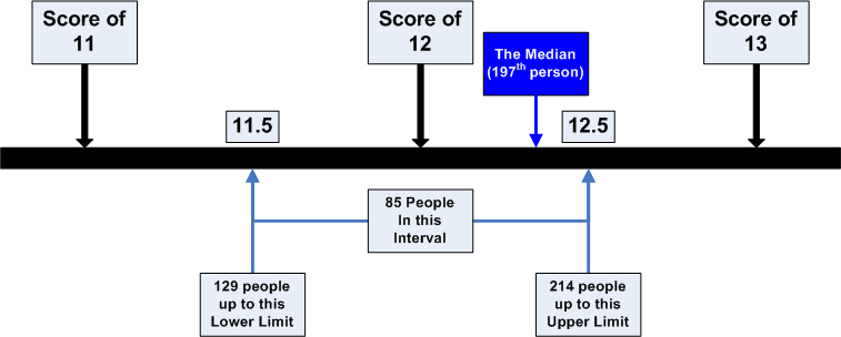
This is the most complicated formula that you have had to deal with so far, but the logic behind it is not as complicated as the formula makes it appear. We have determined that the middle score (197th) appears in the interval of 12, which has real limits from 11.5 to 12.5. Furthermore, we have determined that 85 people are in that interval and 129 score below that interval. This formula makes the assumption that the 85 people scoring in the interval that contains the median are evenly distributed. That is, the first person takes the bottom 1/85th of that interval, the next person takes the next 1/85th of that interval, up to the last person, who takes the top 1/85th of that space. The value "nmedian - nLRL" computes how far we have to count up from the bottom of the interval. In this case, we must count up 68 people [197-129], which is 80% of the way from the bottom of the interval [68/85]. The figure below illustrates this process, which is built into the formula.
Although you can create a frequency distribution and do the computations that we just walked you through, with large data sets, it is much more likely that you will use a computer package like SPSS for Windows to do this computation. Computer packages will use this formula to make the computation. To see how you would request the computation of the median using SPSS for Windows, click on the button below. When you want to return to this page, use the back arrow key on your browser to return.
|
Compute the median using SPSS |
|
USE THE BROWSER'S |
The Mode
The mode is the most frequently occurring score. In a frequency distribution, you compute the mode by looking for the largest number in the frequency column. The score associated with that number is the mode. Using the frequency distribution previously used for computing the median, the largest frequency is 85, and it is associated with a score of 12. Therefore, 12 is the mode.
If you have a grouped frequency distribution, the mode is the midpoint of the interval that contains the largest number of scores. That can create a bit of instability, which we can illustrate with an example.
Suppose that we use the data from the frequency distribution above to create a grouped frequency distribution with an interval width of 2 scores. If we start by grouping 8 and 9 together, we will produce the following grouped frequency distribution.
| Interval | Frequency | Cumulative Frequency |
| 16-17 | 28 | 394 |
| 14-15 | 81 | 366 |
| 12-13 | 156 | 285 |
| 10-11 | 97 | 129 |
| 8-9 | 32 | 32 |
The interval with the largest frequency is 12-13, and the midpoint of that interval is 12.5. Therefore, 12.5 is the mode.
However, suppose that we create a similar grouped frequency distribution, again with an interval of 2, but this time we start with an interval of 7-8. If we do, we will get the following grouped frequency distribution.
| Interval | Frequency | Cumulative Frequency |
| 17-18 | 8 | 394 |
| 15-16 | 53 | 386 |
| 13-14 | 119 | 333 |
| 11-12 | 143 | 214 |
| 9-10 | 60 | 71 |
| 7-8 | 11 | 11 |
Now the interval with the largest frequency is 11-12, with a midpoint of 11.5. Therefore the mode is 11.5. So the mode shifts depending on how we set up the intervals. This effect is rather small in this example, because the sample sizes are rather large and the distribution is close to symmetric.
With small sample sizes and less symmetric distributions, you can get huge shifts in the mode. This is why the mode is considered to be unstable. Another reason that the mode is unstable is that a shift of just a few scores could change the mode by making a different score the mode.
To practice computing the mode using SPSS for Windows, click on the buttons below. To return to this page after viewing the computation, use the browser's back arrow key.
|
Compute the mode using SPSS |
|
USE THE BROWSER'S |
Comparing the Measures
In the textbook, we provide an example in one of the Cost of Neglect boxes of how the mean can misrepresent the typical score when there are a few deviant scores. In our example, there were five employees with the company, four of which made $40,000 and one making $340,000. The mean was $100,000, which clearly does not reflect the typical salary. The median ($40,000) was a much better estimate of the typical salary.
This is an extreme example of a general principle. When a distribution is symmetric, like in the top panel of the figure below, the mean, median, and mode will all be the same. However, as the curve becomes more skewed, these three measures of central tendency diverge. The mode will always be at the peak of the curve, because the highest point indicates the most frequent score. The mean will be pulled the most toward the tail of the skew, with the median in between.
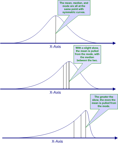
These graphs may help you to understand what each of these measures of central tendency measure.
-
The mode is always the score at which the curve reaches its highest point (i.e., the most frequent score).
-
The median is the score the cuts the curve into two equal areas. In other words, the area above the median line is equal to the area below the median line. The area under a frequency curve is proportional to the number of people or objects represented by that curve. Remember, the median is the 50 percentile, so that should be an equal number above and below the median. So the area of the curve should be equal above and below the median to reflect this.
-
The mean is the balance point for the curve. What that means is if we cut a block of wood in the exact shape of the curve, the mean would be the point at which that block of wood could be perfectly balanced on your finger. It is the point where the average distance from the mean is exactly the same for the scores above the mean and the scores below the mean.