Measures of Variability

Measures of variability indicate the degree to which the scores in a distribution are spread out. Larger numbers indicate greater variability of scores. Sometimes the word dispersion is substituted for variability, and you will find that term used in some statistics texts.

We will divide our discussion of measures of variability into four categories: range measures, the average deviation, the variance, and the standard deviation.

Range Measures

In Chapter 5, we introduced only one range measure, which was called the range. The range is the distance from the lowest score to the highest score. We noted that the range is very unstable, because it depends on only two scores. If one of those scores moves further from the distribution, the range will increase even though the typical variability among the scores has changed little.

This instability of the range has lead to the development of two other range measures, neither of which rely on only the lowest and highest scores. The interquartile range is the distance from the 25th percentile and the 75 percentile. The 25th percentile is also called the first quartile, which means that it divides the first quarter of the distribution from the rest of the distribution. The 75th percentile is also called the third quartile because it divides the lowest three quarters of the distribution from the rest of the distribution. Typically, the quartiles are indicated by uppercase Qs, with the subscript indicating which quartile we are talking about (Q₁ is the first quartile and Q₃ is the third quartile). So the interquartile range can be computed by subtracting Q₁ from Q₃ [i.e., Q₃ -Q₁].

There is a variation on the interquartile range, called the semi-interquartile range or quartile deviation. This value is equal to half of the interquartile range.

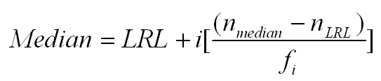
Using this notation, the median is the second quartile (the 50th percentile). That means that we can use a variation of the formula for the median to compute both the first and third quartiles. Looking at the equation below for the median, we would make the following changes to compute these quartiles.

To compute Q₁, n_median becomes n_Q1, which is equal to .25*N. We then identify the interval that contains the n_Q1 score. All of the other values are obtained in the same way as for the median.
To compute Q₃, n_median becomes n_Q3, which is equal to .75*N. We then identify the interval that contains the n_Q3 score. All of the other values are obtained in the same way as for the median.
To compute the interquartile range, subtract Q₁ from Q₃.
To compute the quartile deviation, divide the interquartile range by 2.

It is common to report the range, and many computer programs routinely provide the minimum score, maximum score, and the range as part of their descriptive statistics package. Nevertheless, these are not widely used measures of variability. The same computer programs that give a range, will also provide both a standard deviation and variance. We will be discussing these measures of variability shortly, after we have introduced the concept of the average deviation.

The Average Deviation

The average deviation is not a measure of variability that anyone uses, but it provides an understandable introduction to the variance. The variance is not an intuitive statistic, but it is very useful in other statistical procedures. In contrast, the average deviation is intuitive, although generally worthless for other statistical procedures. So we will use the average deviation to introduce the concept of the variance.

The average deviation is, as the name implies, the average deviation (distance) from the mean. To compute it, you start by computing the mean, then you subtract the mean from each score, ignoring the sign of the difference, and sum those differences. You then divide by the number of scores (N). The formula is shown below. The vertical lines on either side of the numerator indicate that you should take the absolute value, which converts all the differences to positive quantities. Therefore, you are computing deviations (distances) from the mean.

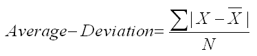
Chapter 5 in the textbook walked you through the computation of the average deviation. The reason we take the absolute value of these distances from the mean is that the sum of the differences from the mean, some positive and some negative, will always equal zero. We can prove that fact with a little algebra, but you can take our word for it.

As we mentioned earlier, the average deviation is easy to understand, but it has little value for inferential statistics. In contrast, the next two measures (variance and standard deviation) are useful in other statistical procedures. So we now turn our attention to them.

The Variance

The variance takes a different approach to making all of the distances from the mean positive so that they will not sum to zero. Instead of taking the absolute value of the difference from the mean, the variance squares all of those differences.

The notation that is used for the variance is a lowercase s². The formula for the variance is shown below. If you compare it with the formula for average deviation, you will see two differences instead of one between these formulas. The first is that the differences are squared instead of taking the absolute value. The numerator of this formula is called the sum of squares, which is short for sum of squared differences from the mean. See if you can spot the second difference.

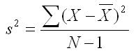
Did you recognize that the variance formula does not divide by N, but instead divides by N-1? The denominator (N-1) in this equation is called the degrees of freedom. It is a concept that you will hear about again and again in statistics. If you would like to know more about degrees of freedom, you can click on this link. This link provides a conceptual explanation of this concept.

The reason that the variance formula divides the sum of squared differences from the mean by N-1 is that dividing by N would produce a biased estimate of the population variance, and that bias is removed by dividing by N-1. You can learn more about the concept of biased versus unbiased estimates of population parameters by clicking on this link.

The Standard Deviation

The variance has some excellent statistical properties, but it is hard for most students to conceptualize. To start with, the unit of measurement for the mean is the same as the unit of measurement for the score. For example, if we compute the mean age of our sample and find that it is 28.7 years, that mean is on the same scale as the individual ages of our participants. But the variance is in squared units. For example, we might find that the variance is 100 years².

Can you even imagine what the unit of years squared represents? Most people can't. But there is a measure of variability that is in the same units as the mean. It is called the standard deviation, and it is the square root of the variance (see the formula below). So if the variance was 100 years², the standard deviation would be 10 years. Since we used the symbol s² to indicate variance, you might not be surprised that we use the lowercase letter s to indicate the standard deviation. You will see in our discussion of relative scores how valuable the standard deviation can be.

At this point, many students assume that the variance is just a step in computing the standard deviation, because the standard deviation seems like it is much more useful and understandable. In fact, you will use the standard deviation for description purposes only and will use the variance for all your other statistical tasks. If you are wondering why that is, click on this link to find out.

Finally, if you want to see how to compute the variance and/or standard deviation by hand or using SPSS for Windows, click on one of the buttons below for those units.

Compute the variance and
standard deviation by hand

Compute the variance and
standard deviation using SPSS

USE THE BROWSER'S
BACK ARROW KEY TO RETURN

Go to the Next Page