 Graziano & Raulin
Research Methods (9th edition)
Comparing Two Correlated Samples
Chapter 11 of the text introduced the concept of correlated groups designs, which can be either within-subjects or matched-subjects designs. These designs require a different statistical procedure for analysis, which is the focus of this section. We will assume initially that we are analyzing a within-subjects design with two groups. At the end of this section, we will talk about how you approach the analysis of a matched-subjects design.
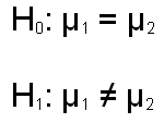
Conceptually, the logic of comparing two correlated groups of participants is identical to the logic of comparing two independent groups of participants. The null and alternative hypotheses (shown below) are identical in both cases. The basic structure of the t-test is identical, in that you are taking the mean difference of the samples, subtracting the mean difference of the population (which is equal to zero under the null hypothesis), and you are dividing this value by the standard error of the difference.
However, as you learned in Chapter 11, the value of the within-subjects design is that it removes the portion of the error term that is due to individual differences. The result is an increase in the power to detect group differences when they exist.
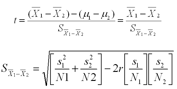
Formulas for computing a t-test for correlated groups are shown below. This test is also referred to as the direct difference t-test or the correlated t-test. Again, like the null and alternative hypotheses, the formula for computing the t is identical to the formula used in the two independent groups situation. The only difference comes in how the standard error of the mean difference is computed.
The second equation shows how this standard error is computed. This equation can be written in many algebraically identical ways, but this variation illustrates the value of the within-subjects design. The term in the first bracket under the square root sign is essentially the standard error in the independent groups design. There is a small and subtle difference between how this term is computed here and how it is computed in the independent groups design, but we can overlook this fairly trivial difference for this argument.
The second term under the square root sign (starting with 2r) is how much we can reduce the error term because the correlated groups design controls for individual differences. The correlation here (r) is the correlation between the dependent measures in the two conditions. If that correlation is high, it means that people tend to be consistent across conditions and that there are considerable individual differences in overall performance. If that is the case, a within-subjects design will increase power dramatically. If the correlation is low, it means that people are not consistent across conditions, and thus the effect of individual differences is not terribly large. Consequently, the increase in power is less.
There are examples elsewhere on this website on how to compute the t-test for correlated groups either manually or using SPSS for Windows. Simply click on the links below to see those examples and use the back arrow key on your browser to return to this section when you are done.
|
Compute the t-test for correlated samples by hand |
|
Compute the t-test for correlated samples using SPSS |
|
USE THE BROWSER'S |
You learned in Chapter 11 that a matched-subjects design involves matching participants on critical variables and then randomly assigning one member of each matched set to each of the groups of a study. The result is that there are different people in each group, like we have in the independent groups design. However, these people are not independent of one another because of the matching. Therefore, you DO NOT use the t-test for independent groups introduced in the previous section. Instead, you use the t-test introduced in this section and treat the matched pairs of participants as if they were the same person. In a matched-subjects design, you must keep track of who is matched with who all the way to the analysis stage.