 Graziano & Raulin
Research Methods (9th edition)
Testing One Sample with a t-Test
This section will introduce you to statistical hypothesis testing. We will be testing a hypothesis about whether a sample mean came from a particular population. We will be looking at two similar and related procedures.
Testing a Sample Against a Known Population
The simplest form of a statistical test is to compare a sample to see if it came from a population with known population parameters. It is a very rare situation in which such population parameters are known, but it is an easier statistical procedure to compute. Therefore, we will start here, which will provide a basis for understanding the logic of statistical hypothesis testing.
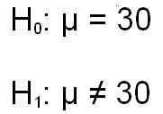
For example, suppose that we know that the population mean and standard deviation for a given variable are 30.00 and 4.00, respectively. The null hypothesis is that our sample came from a population with a population mean of 30, and the alternative hypothesis is that the population mean for our sample is not equal to 30, as shown below.
This form of the null and alternative hypotheses are said to be nondirectional in that the alternative hypothesis does not state whether the the population mean is either greater than or less than 30, only that it is not equal to 30. Shortly, you will learn about directional hypotheses.
We can draw this situation graphically even before we take a look at our obtained mean. Let us assume that the sample mean is based on a sample size that is sufficiently large that the central limit theorem applies. For this example, we will assume that the sample size is 100. Therefore, we know that the sampling distribution of means will be normal.
We can compute the standard error of the mean (that is, the standard deviation for this sampling distribution of means) by dividing the population standard deviation by the square root of the sample size, as you learned previously. In this case, the standard error is equal to 4.00 divided by the square root of 100, which is .40. (Check the math to make sure you understand how this is computed.)
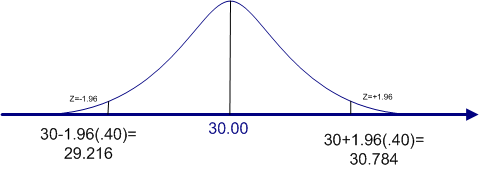
You also learned previously that in statistical tests, we set a decision criterion called alpha. For now, let's assume that we have set alpha to the traditional value of .05. When we are testing a nondirectional hypothesis, as we are here, we need to split the value of .05 between the two tails of the distribution so that there is .025 in each tail. This may sound familiar, because we performed this task before when we computed a confidence interval. There you learned that 1.96 standard deviations above the mean will cut off the top 2.5%, and a 1.96 standard deviations below the mean will cut off the bottom 2.5%.
The figure below illustrates the sampling distribution for means for the example we are working on here. So if our sample mean is less than 29.216 or greater than 30.784, it is not likely to have come from a population with a mean of 30.00 and a standard deviation of 4.00. So we would reject the null hypothesis and conclude that our mean must have come from another population with a different population mean. We could be wrong, but 95% of the time we will be correct. Setting the alpha at .05 says that we have to be at least 95% confident of our decision before we reject the null hypothesis.
Suppose that we want to be even more confident of our decision before we reject the null hypothesis. In that case, we might set the alpha level to .01, which says that we want to be 99% confident of our decision before rejecting the null hypothesis. If we assume the nondirectional hypotheses above, we will need to find a value that will cut off .005 of the area in each tail (half of .01).
If you consult the standard normal table, you will find the a Z-score of 2.58 cuts off the top .005 of the distribution. So our confidence interval will be modified as shown below, with the decision points moving out a bit further from the decision points for an alpha of .05. The new decision points are 28.968 and 31.032, as shown in the figure below. If our sample mean falls outside of those limits, we would consider that convincing enough evidence that we should reject the null hypothesis.

These two examples rest on the assumption that the alternative hypothesis is nondirectional. When we make a nondirectional hypothesis, we must split the area under the curve that is equal to alpha evenly among the two tails of the distribution. We refer to such a situation as a two-tail probability or a two-tail test.
However, you may have a strong reason to believe that the alternative hypothesis should be directional. Instead of the alternative hypothesis reading that the population mean is not equal to 30, it reads that the population mean is greater than 30. Such a directional hypothesis is called a one-tail test, because the entire value of alpha is concentrated in the one tail.
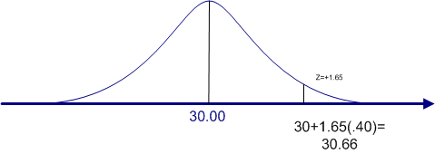
For example, if alpha is .05, we would find the value of Z that cuts off the top 5% (.05) in the upper tail. We do not need to split the alpha because we are predicting that, if the null hypothesis is rejected, it must be because the population mean is actually larger than 30. Again, we consult the standard normal table to find the value of Z that cuts off the top 5%. If you do that, you will find that a Z of 1.64 cuts of .0505 and a Z of 1.65 cuts off .0495. So the Z that would cut off exactly .0500 is half way between 1.64 and 1.65, or 1.645. This is probably more precision than we need for most decisions. The norm is to take the most conservative figure, which is the Z score that comes closest to the alpha level but does not exceed it, which in this case is 1.65.
This situation is graphed in the figure below. The cutoff for rejecting the null hypothesis is 30.66. If the sample mean is greater than 30.66, we reject the null hypothesis and conclude that the population mean must be greater than 30.
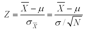
These figures and the above explanation will help you to visualize the conceptual process behind this first inferential statistic that we are covering, but the procedures require more computation than is necessary. Instead of computing the cutoff scores, all we really need to compute is the Z-score for our sample mean, which we can do using the formula below. Then we evaluate that Z-score against the critical Z-score, which is the Z-score that we would use to reject the null hypothesis. For example, if we are testing a nondirectional hypothesis with an alpha of .05, the critical value of Z is ±1.96 (read plus or minus 1.96). We use the plus or minus (±) designation, because in a nondirectional test, sample means that are either too large or too small will result in us rejecting the null hypothesis. Similarly, the critical value of Z for a nondirectional test with an alpha of .01 is ±2.58. [Although not necessary, we recommend that you draw a figure like the ones above at least the first few times that you perform this inferential statistic to help you visual what you are doing.]
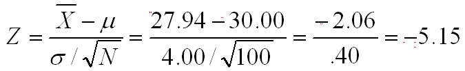
So going back to our original situation, we want to test the null hypothesis that the population value is equal to 30.00. We know that the population standard deviation is 4.00. If we conduct a nondirectional test (i.e., a two-tail test) with an alpha of .05, our critical values of Z are ±1.96. If the mean of our sample of 100 people is 27.94, is this sufficiently different from our population mean of 30.00 to reject the null hypothesis and conclude that the sample must have been drawn from a different population with a different population mean?
Plugging the numbers into the formula above, we get a computed value of Z of -5.15. This value certainly exceeds our critical value of ±1.96, so we reject the null hypothesis and conclude that our sample was not drawn from this population.
Testing a Sample Against a Hypothesized Population
It is actually rare to know the population parameters. The more common situation is when we want to test a sample mean against a hypothesized population mean. In this situation, we have to estimate the population standard deviation using the standard deviation from the sample. We have done this estimation before. The trick was to use a formula that would give an unbiased estimate of the population parameter. So our formula will change slightly in this situation.
But there is one more important change in this situation, and this change involves introducing a new distribution, called the Student's t distribution, or simply the t distribution. Actually, the t distribution is an entire family of distributions, all of which are a bit flatter and more spread out than normal distribution, as illustrated in the figure below. How much flatter and more spread out a t distribution is will depend on the number of degrees of freedom.
You were introduced to the concept of degrees of freedom (df) earlier, and you also learned earlier that dividing by the degrees of freedom instead of N produced an unbiased estimate of the population variance. Here we are using the concept of df to identify the appropriate t distribution to use in this statistical test.
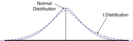
It is helpful to understand how the t distributions compare to the standard normal distribution. The larger the sample size, the closer the t distribution is to the standard normal or Z distribution. In fact, when the sample size is infinity, the t and Z distributions are identical. But as the sample size gets smaller, the t distribution becomes progressively flatter and more spread out.
Because there are so many t distributions, what is tabled is not each distribution, but rather the critical values for each distribution. Click on this link to view the t distribution table. Note that this table presents critical values for various alpha levels (labeled level of significance in the table) ranging from .20 to .001 and for various degrees of freedom (df).
When we are testing a single sample against a hypothesized population mean, the degrees of freedom are one less than the sample size (i.e., df = N-1). If you look at the bottom of the table, where the dfs are equal to infinity, you will find some familiar numbers (1.645 for level of significance of .10, 1.96 for .05, and 2.58 for .01). These were the critical values of Z that we identified earlier on this page.
Note that if you are using a one-tail test, the alpha is not split between the tails. Hence, you look up the critical value that is double the level of significance of the two-tail test. So a one-tail test with an alpha of .05 is equivalent to a two-tail test with an alpha of .10.
Note also that as the degrees of freedom decrease, the critical value at any level of significance increases. The reason is that with smaller sample sizes, the t distribution is progressively flatter and more spread out, so you have to go further out into the tail to cut off a given area of the curve. This effect is very dramatic for small sample sizes, but much less dramatic for moderate to large sample sizes.
For example, let's take the two tail alpha value of .05. At infinity, the critical value is 1.96, but it only increases to 1.98 at df=120 and 2.00 at df=60. However, by the time that you reach df=10, the critical value is 2.228, at df=5, it is 2.571, and at df=1, it is 12.706. If the degrees of freedom are equal to 1, the sample size is 2, which is the minimum N for which we can compute a variance estimate. But with sample sizes that small, population estimates are not going to be precise. This general concept was first introduced when we talked about the standard error of the mean. The larger the sample size (and therefore the dfs), the more confident we can be in our population estimates, and therefore the less we have to adjust our critical values of t to compensate for the imprecision of our population estimates.
The t-test comparing a sample against a hypothesized population mean is called a one-sample t-test or a single-group t-test.
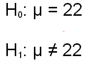
Now that you have the basic concepts for the single-group t-test, let's actually work through a problem. Let's assume that you have a sample of 15 people, and the mean and standard deviation of that sample are 24.33 and 6.29, respectively. You want to test the hypothesis that the population mean for the population from which this sample was drawn is 22.00. Let's further assume that you decide to conduct a two-tail test with the traditional alpha level of .05.
Listed below are the null and alternative hypotheses. The formula that you would use to compute the value of t is virtually identical to the formula that is used to compute the Z when the population standard deviation is known. The only difference is that we substitute the unbiased estimate of the population standard deviation for the actual population standard deviation. The next formula shows the actual computations.
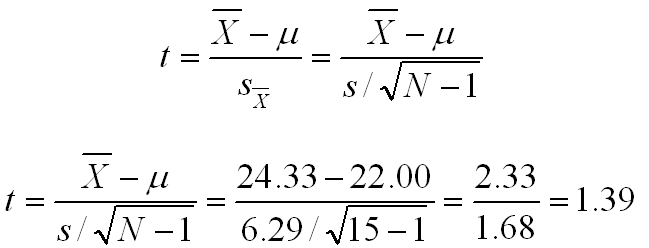
The computed value of t (1.39) needs to be compared to the critical value of t for the alpha level and degrees of freedom. Since the sample size is 15, df=14. Looking at the t distribution table in the column labeled .05 level of significance (equivalent to a two-tail test with an alpha of .05). If you do, you will find that the critical value of t is 2.145. Since our computed value of t is less than this critical value, we fail to reject the null hypothesis and we conclude that this sample may have come from a population with a population mean of 22.00.