 Graziano & Raulin
Research Methods (9th edition)
Computational Procedures
for a One-Way ANOVA
In this example, we will compute a one-way ANOVA for data from three independent groups. The raw data for the 16 subjects are listed below. Note that this is a between-subjects design, so different people appear in each group.
The Raw Data
Here are the raw data from the three groups (6 people in Group 1, and 5 each in Groups 2 and 3).
| Group 1 | Group 2 | Group 3 |
| 3 | 4 | 9 |
| 1 | 3 | 7 |
| 3 | 5 | 8 |
| 2 | 5 | 11 |
| 4 | 4 | 9 |
| 3 |
The first step in the computation is to add the scores in each column and compute the sum of the squared scores for each column. We also count the number of scores in each column, compute the mean by dividing the sum by the number of scores, and compute the sum of squares.
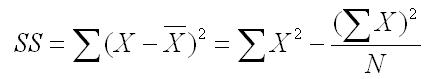
We defined the sum of squares in Chapter 5 as the average squared deviation from the mean. However, there is an easier computational formula for the SS, which you learned in the section of this website that showed you how to compute the variance. Listed below is both the definitional formula (first part) and the computational formula (second part).
Summary Statistics
We have done the computations described above for each of the three groups and organized them in three columns. We have also included a fourth column to put the total scores, total sum of X2, and total sample size, all of which will also be needed for the computations. In this way, we have all of the values that we will need for the computation of a one-way ANOVA at our fingertips.
| Group 1 | Group 2 | Group 3 | Totals | |
| Sum of X | 16 | 21 | 44 | 81 |
| Sum of X2 | 48 | 91 | 396 | 535 |
| n | 6 | 5 | 5 | 16 |
| Mean | 2.67 | 4.20 | 8.80 | |
| SS | 5.33 | 2.80 | 8.80 |
Compute the SSs for the ANOVA
The formulas for computing the three sums of squares (between, within, and Total) are shown below, with the numbers plugged in. The notation may look complicated, but all of the needed values can be found in the summary table that we just prepared. The only real new terminology uses summation notation in which we sum across the groups (i, which refers to the group number, goes from 1 to k, which is the number of groups). We use this notation because we can have any number of groups in a design like this and we want a formula that will describe what we should do regardless of how many groups we have.
Most students find it easier to understand the notation by looking at the formula and see where the numbers for the formula can be found in the summary table above. We have used more parentheses than actually needed algebraically to specify what needs to be done. The rule is that you always do things inside a parenthesis before you do things outside of the parenthesis. If you remember that simple rule, you will not have to remember the more complicated algebraic rules about what computations should be done first.
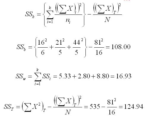
Double check the computation of the SSs by seeing if they add up. SST = SSb + SSw = 108.00 + 16.93 = 124.93 [There is a slight difference here due to rounding error.]
Fill in the Summary Table
The dfb is equal to the number of groups (k) minus 1. The dfw is equal to the total number of participants minus the number of groups (N - k). The dfT is equal to the total number of participants (N) minus 1. Note that the dfT is equal to the dfb plus the dfw in the same way that the SST is equal to the sum of the SSb and SSw.
The MSs are computed by dividing the SSs by their respective dfs, and the F is computed by dividing the MSb by the MSw. All of these values have been inserted into the standard summary table for ANOVA below.
| Source | df | SS | MS | F |
| Between | 2 | 108.00 | 54.00 | 41.46 |
| Within | 13 | 16.93 | .30 | |
| Total | 15 | 124.94 |
The final step is to compare the value of the F computed in this analysis with the critical value of F in the F Table. You look up the critical value by using the degrees of freedom. In our case, the dfb is 2 and the dfw is 13. The critical value of F for an alpha of .05 is 3.80. Since our obtained F exceeds this value, we reject the null hypothesis and conclude that there is a significant difference between the groups.