 Graziano & Raulin
Research Methods (9th edition)
Computational Procedures
for a Factorial ANOVA
The Raw Data
If one needed convincing about the advantages of using computers to calculate statistical procedures, doing a factorial ANOVA by hand will definitely convince you. Nevertheless, it can be instructive to compute a few complex ANOVAs to get a feel for the procedures. We will run through a basic two-way ANOVA, in which both factors are between-subjects factors. Please note that the formulas and procedures change dramatically if one of both factors are within-subjects factors.
It is critically important in complex computations to organize all of your work, starting with organizing the data. In our hypothetical example, we have two factors (A and B), and each factor has three levels. The data set is small (4 to 5 participants in each of the 9 groups). It is common to have 20 or more participants in each group in a real study. We have systematically arranged the data in nine columns as shown in the table below. This facilitates the computation of key terms that will be used later in the ANOVA.
| B1 | B2 | B3 | ||||||||
| A1 | A2 | A3 | A1 | A2 | A3 | A1 | A2 | A3 | ||
| 10 | 7 | 11 | 1 | 6 | 4 | 3 | 2 | 5 | ||
| 8 | 4 | 9 | 2 | 7 | 3 | 2 | 1 | 6 | ||
| 7 | 3 | 10 | 1 | 6 | 6 | 3 | 2 | 4 | ||
| 9 | 2 | 9 | 4 | 5 | 4 | 3 | 3 | 5 | ||
| 6 | 1 | 2 | 3 | 4 | 5 | |||||
Summary Statistics
Just like in the one-way ANOVA, our next step is to compute several terms for each of the columns of data. Because this is a factorial ANOVA, however, it facilitates later computation by organizing these computed terms as factors. Therefore, we will organize these components as a 3 X 3 matrix, with row and column totals computed for many (but not all) of the terms in this matrix.
The table below shows these computations. For each column of scores, we will compute the sum, the sum of squared values, the number of scores (n), the sum of squares (SS), the mean, and a value that is the sum of the column, which is then squared and divided by n [we will write it as (sum of X)2/n].
[Note that throughout this presentation, we will be using the phrase "sum of" instead of the Greek letter Sigma, because some browsers do not correctly interpret symbols that are not part of a limited character set. The formulas will use the familiar notation. We are trying to avoid anything in this material that will not be reproduced the way we intended it for every student, no matter what computer or browser that student might be using.]
| | | B Levels | | | |||||
| A Levels | Terms | | | B1 | B2 | B3 | | | Totals |
| sum of X | | | 40 | 16 | 50 | | | 106 | |
| sum of X2 | | | 330 | 78 | 504 | | | 912 | |
| A1 | n | | | 5 | 4 | 5 | | | 14 |
| SS | | | 10 | 14 | 4 | | | ||
| (sum of X)2/n | | | 320 | 64 | 500 | | | 802.57 | |
| mean | | | 8 | 4 | 10 | | | 7.57 | |
| --------- | -------------- | | | ----------- | ----------- | ----------- | | | ----------- |
| sum of X | | | 10 | 24 | 20 | | | 54 | |
| sum of X2 | | | 26 | 146 | 86 | | | 258 | |
| A2 | n | | | 5 | 4 | 5 | | | 14 |
| SS | | | 6 | 2 | 6 | | | ||
| (sum of X)2/n | | | 20 | 144 | 80 | | | 208.29 | |
| mean | | | 2 | 6 | 4 | | | 3.86 | |
| --------- | -------------- | | | ----------- | ----------- | ----------- | | | ----------- |
| sum of X | | | 15 | 8 | 25 | | | 48 | |
| sum of X2 | | | 47 | 18 | 127 | | | 192 | |
| A3 | n | | | 5 | 4 | 5 | | | 14 |
| SS | | | 2 | 2 | 2 | | | ||
| (sum of X)2/n | | | 45 | 16 | 125 | | | 164.57 | |
| mean | | | 3 | 2 | 5 | | | 3.43 | |
| --------- | -------------- | | | ----------- | ----------- | ----------- | | | ----------- |
| sum of X | | | 65 | 48 | 95 | | | 106 | |
| sum of X2 | | | 403 | 242 | 717 | | | 1362 | |
| Totals | n | | | 15 | 12 | 15 | | | 42 |
| SS | | | | | 331.90 | ||||
| (sum of X)2/n | | | 281.67 | 192.00 | 601.67 | | | 1030.10 | |
| mean | | | 4.33 | 4.00 | 6.33 | | | 4.95 |
Please note how the row and column totals are computed. The values of sum of X, sum of X2, and n are computed by adding across the rows or adding down the columns. In contrast, the values of (sum of X)2/n and the mean are computed using the appropriate row and column totals, in the same way that those values were computed within the cells.
For example, the sum of X, sum of X2, and n for all of the participants tested under A1 is computed by summing horizontally across the various levels of B (near the top of the above table). These total values are 106, 912, and 14 respectively. However, the values for SS, (sum of X)2/n, and the mean are NOT computed by summing across the levels of A1, but rather use the values that were computed by summing across A1. For example, the mean is equal to the sum of X divided by n.
We could compute the SS for the row and column totals, but there is no need to because it will not be used in any of the later computations. Note that we did compute the SS value for the grand total (lower right cell) because this will be used later. The grand total is computed by summing across all participants, no matter what combination of conditions the participants were tested under. In our table, we can sum across the totals to the the sum of X, the sum of X2, and n and then use those values to get the other three terms.
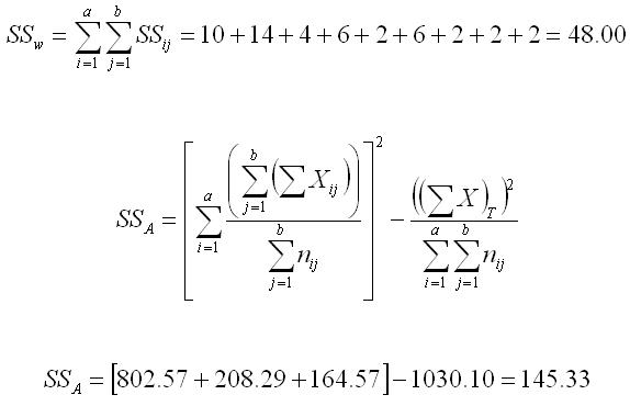
Computing the Sums of Squares
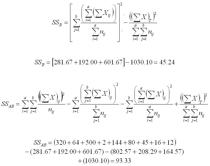
Listed below are the computations for the various SSs that are a part of the two-way ANOVA. The notation is rather complex and forbidding at first. The SSw is simply the sum of each of the SS from the 9 individual cells. The SSA is the sum of the {(sum of X)2/n} terms across the three levels of Factor A minus that same term from the grand total cell (in the lower right hand corner of the above table). The SSB is computed in the same way using the values for Factor B. Finally, the SSAB is equal to the sum of the {(sum of X)2/n} terms for all nine cells, minus those same terms for both the row and column totals, plus that same term for the grand total. We had already computed the SST in our table above. Are you convinced now that computers really make this a LOT easier?
Computing the F-Ratios
The bulk of the computational work is now complete. To compute the F-ratios, we set up the summary table for the ANOVA. The degrees of freedom for Factors A and B are equal to the number of levels of each factor minus 1. The degrees of freedom for the interaction (AB) is equal to the product of the degrees of freedom for the individual factors. The degrees of freedom within-groups is equal to the total number of participants minus the number of cells. Finally, the degrees of freedom total is equal to the total number of participants minus 1.
Our next step is to insert the Sums of Squares computed above into the summary table, compute the Mean Squares by dividing each sum of squares by its respective degrees of freedom, and finally computing the F-ratios by dividing each Mean Square by the Mean Square within-groups. All of these values are shown in the Table below.
Summary Table
| Source | df | SS | MS | F |
| Factor A | 2 | 145.33 | 72.67 | 49.96 |
| Factor B | 2 | 45.24 | 22.62 | 15.55 |
| AB Interaction | 4 | 93.33 | 23.33 | 16.04 |
| Within-Groups | 33 | 48.0 | 1.45 | |
| Total | 41 | 331.90 |
The final step is to compare the value of the F computed in these analyses with the critical values of F in the F Table. You look up the critical values by using the degrees of freedom. In our case, the dfA and dfB are both 2, the dfAB is 4, and the dfw is 33. The critical value of F for an alpha of .05 is 3.29 for the two main effects and 2.66 for the interaction.
Since our obtained Fs exceed these values, we reject the null hypothesis in all cases. We conclude that there is a significant main effect for Factor A, a significant main effect for Factor B, and a significant AB interaction.
Remember our admonition from the text: When you have both main effects and interactions, you should interpret the main effects in terms of the interaction.