 Graziano & Raulin
Research Methods (9th edition)
Measures of Relationship
Chapter 5 of the textbook introduced you to the three most widely used measures of relationship: the Pearson product-moment correlation, the Spearman rank-order correlation, and the Phi correlation. We will be covering these statistics in this section, as well as other measures of relationship among variables.
What is a Relationship?
Correlation coefficients are measures of the degree of relationship between two or more variables. When we talk about a relationship, we are talking about the manner in which the variables tend to vary together. For example, if one variable tends to increase at the same time that another variable increases, we would say there is a positive relationship between the two variables. If one variable tends to decrease as another variable increases, we would say that there is a negative relationship between the two variables. It is also possible that the variables might be unrelated to one another, so that you cannot predict one variable by knowing the level of the other variable.
As a child grows from an infant into a toddler into a young child, both the child's height and weight tend to change. Those changes are not always tightly locked to one another, but they do tend to occur together. So if we took a sample of children from a few weeks old to 3 years old and measured the height and weight of each child, we would likely see a positive relationship between the two.
A relationship between two variables does not necessarily mean that one variable causes the other. When we see a relationship, there are three possible causal interpretations. If we label the variables A and B, A could cause B, B could cause A, or some third variable (we will call it C) could cause both A and B.
With the relationship between height and weight in children, it is likely that the general growth of children, which increases both height and weight, accounts for the observed correlation. It is very foolish to assume that the presence of a correlation implies a causal relationship between the two variables. There is an extended discussion of this issue in Chapter 7 of the text.
Scatter Plots and Linear Relationships
A helpful way to visualize a relationship between two variables is to construct a scatter plot, which you were briefly introduced to in our discussion of graphical techniques. A scatter plot represents each set of paired scores on a two dimensional graph, in which the dimensions are defined by the variables.
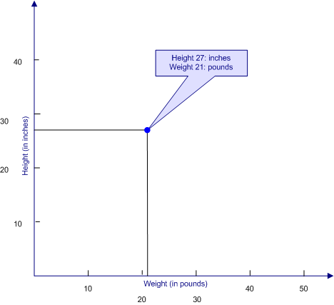
For example, if we wanted to create a scatter plot of our sample of 100 children for the variables of height and weight, we would start by drawing the X and Y axes, labeling one height and the other weight, and marking off the scales so that the range on these axes is sufficient to handle the range of scores in our sample. Let's suppose that our first child is 27 inches tall and 21 pounds. We would find the point on the weight axis that represents 21 pounds and the point on the height axis that represents 27 inches. Where these two points cross, we would put a dot that represents the combination of height and weight for that child, as shown in the figure below.
We then continue the process for all of the other children in our sample, which might produce the scatter plot illustrated below.
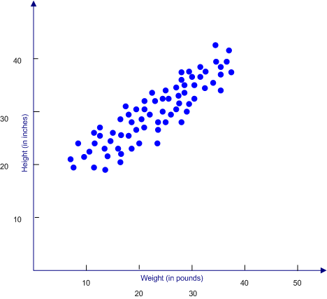
It is always a good idea to produce scatter plots for the correlations that you compute as part of your research. Most will look like the scatter plot above, suggesting a linear relationship. Others will show a distribution that is less organized and more scattered, suggesting a weak relationship between the variables. But on rare occasions, a scatter plot will indicate a relationship that is not a simple linear relationship, but rather shows a complex relationship that changes at different points in the scatter plot.
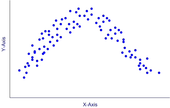
The scatter plot below illustrates a nonlinear relationship, in which Y increases as X increases, but only up to a point; after that point, the relationship reverses direction. Using a simple correlation coefficient for such a situation would be a mistake, because the correlation cannot capture accurately the nature of a nonlinear relationship.
Pearson Product-Moment Correlation
The Pearson product-moment correlation was devised by Karl Pearson in 1895, and it is still the most widely used correlation coefficient. This history behind the mathematical development of this index is fascinating. Those interested in that history can click on the link. But you need not know that history to understand how the Pearson correlation works.
The Pearson product-moment correlation is an index of the degree of linear relationship between two variables that are both measured on at least an ordinal scale of measurement. The index is structured so the a correlation of 0.00 means that there is no linear relationship, a correlation of +1.00 means that there is a perfect positive relationship, and a correlation of -1.00 means that there is a perfect negative relationship.
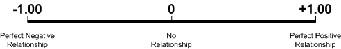
As you move from zero to either end of this scale, the strength of the relationship increases. You can think of the strength of a linear relationship as how tightly the data points in a scatter plot cluster around a straight line. In a perfect relationship, either negative or positive, the points all fall on a single straight line. We will see examples of that later.
The symbol for the Pearson correlation is a lowercase r, which is often subscripted with the two variables. For example, rxy would stand for the correlation between the variables X and Y.
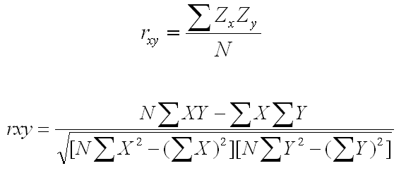
The Pearson product-moment correlation was originally defined in terms of Z-scores. In fact, you can compute the product-moment correlation as the average cross-product Z, as show in the first equation below. But that is an equation that is difficult to use to do computations. The more commonly used equation now is the second equation below.
Although this equation looks much more complicated and looks like it would be much more difficult to compute, in fact, this second equation is by far the easier of the two to use if you are doing the computations with nothing but a calculator.
You can learn how to compute the Pearson product-moment correlation either by hand or using SPSS for Windows by clicking on one of the buttons below. Use the browser's return arrow key to return to this page.
|
Compute the Pearson product-moment |
|
Compute the Pearson product-moment |
|
USE THE BROWSER'S |
Spearman Rank-Order Correlation
The Spearman rank-order correlation provides an index of the degree of linear relationship between two variables that are both measured on at least an ordinal scale of measurement. If one of the variables is on an ordinal scale and the other is on an interval or ratio scale, it is always possible to convert the interval or ratio scale to an ordinal scale. That process is discussed in the section showing you how to compute this correlation by hand.
The Spearman correlation has the same range as the Pearson correlation, and the numbers mean the same thing. A zero correlation means that there is no relationship, whereas correlations of +1.00 and -1.00 mean that there are perfect positive and negative relationships, respectively.
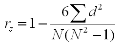
The formula for computing this correlation is shown below. Traditionally, the lowercase r with a subscript s is used to designate the Spearman correlation (i.e., rs). The one term in the formula that is not familiar to you is d, which is equal to the difference in the ranks for the two variables. This is explained in more detail in the section that covers the manual computation of the Spearman rank-order correlation.
|
Compute the Spearman rank-order |
|
Compute the Spearman rank-order |
|
USE THE BROWSER'S |
The Phi Coefficient
The Phi coefficient is an index of the degree of relationship between two variables that are measured on a nominal scale. Because variables measured on a nominal scale are simply classified by type, rather than measured in the more general sense, there is no such thing as a linear relationship. Nevertheless, it is possible to see if there is a relationship.
For example, suppose you want to study the relationship between religious background and occupations. You have a classification systems for religion that includes Catholic, Protestant, Muslim, Other, and Agnostic/Atheist. You have also developed a classification for occupations that include Unskilled Laborer, Skilled Laborer, Clerical, Middle Manager, Small Business Owner, and Professional/Upper Management. You want to see if the distribution of religious preferences differ by occupation, which is just another way of saying that there is a relationship between these two variables.
The Phi Coefficient is not used nearly as often as the Pearson and Spearman correlations. Therefore, we will not be devoting space here to the computational procedures. However, interested students can consult advances statistics textbooks for the details. you can compute Phi easily as one of the options in the crosstabs procedure in SPSS for Windows. Click on the button below to see how.
| Using Crosstabs in SPSS for Windows |
| USE THE BROWSER'S BACK ARROW KEY TO RETURN |
Advanced Correlational Techniques
Correlational techniques are immensely flexible and can be extended dramatically to solve various kinds of statistical problems. Covering the details of these advanced correlational techniques is beyond the score of this text and website. However, we have included brief discussions of several advanced correlational techniques on this Student Resource Website, including multidimensional scaling, path analysis, taxonomic search techniques, and statistical analysis of neuroimages.
Nonlinear Correlational Procedures
The vast majority of correlational techniques used in psychology are linear correlations. However, there are times when we can expect to find nonlinear relationships and we would like to apply statistical procedures to capture such complex relationships. This topic is far too complex to cover here. The interested student will want to consult advanced statistical textbooks that specialize in regression analyses.
There are two words of caution that we want to state about using such nonlinear correlational procedures. Although it is relatively easy to do the computations using modern statistical software, you should not use these procedures unless you actually understand them and their pitfalls. It is easy to misuse the techniques and to be fooled into believing things that are not true from a naive analysis of the output of computer programs.
The second word of caution is that there should be a strong theoretical reason to expect a nonlinear relationship if you are going to use nonlinear correlational procedures. Many psychophysiological processes are by their nature nonlinear, so using nonlinear correlations in studying those processes makes complete sense. But for most psychological processes, there is no good theoretical reasons to expect a nonlinear relationship.